Segmentation - a different approach
Background
This high-level, code-free tutorial explains the main steps of the Thaumato Anakalyptor 1 pipeline for automated segmentation in full 3D.
For a more technical walkthrough of the pipeline, see this walkthrough video.
For an introduction to one of the core problems in this pipeline where we need your help, check out the Sheet Stitching Problem Playground.
Thaumato is one approach but there may be others - for example, volumetric instance segmentation might be useful as an input to later mesh stitching algorithms. If interested, check out this notebook providing easy access to volumetric segmentation labels.
Walkthrough
We will tackle the task of segmentation from another perspective: that of a Neapolitan fisherman.

As we saw in the "Segmentation and Flattening" tutorial, the ultimate purpose of segmentation is that of identifying a triangular mesh on the wrapped papyrus sheet.
Imagine being Neapolitan fishermen, casting our nets not into schools of fish... but onto sheets! We want the net to adhere perfectly on the inner part of the sheet, that is next to where ink is supposed to be located. Indeed, the ink lies on the face of the papyrus that looks towards the pole of rotation of the scroll.
Here, adherence means every node of the net should be placed on the inner surface of the sheet, with adjacent nodes also being adjacent on the sheet. Therefore the problem is twofold: node placement and connectivity establishment.
But how can we cast the net in? After all, the data we have is a 3D volumetric image composed of colored blocks. You can think of it as a big volume made of single units of grayscale LEGO blocks (Figure 1, left). The color of a block represents the density of the material in that region of space: lighter means more dense, hence could be papyrus, while darker means less dense, and could be air. The ink is somewhere in there.
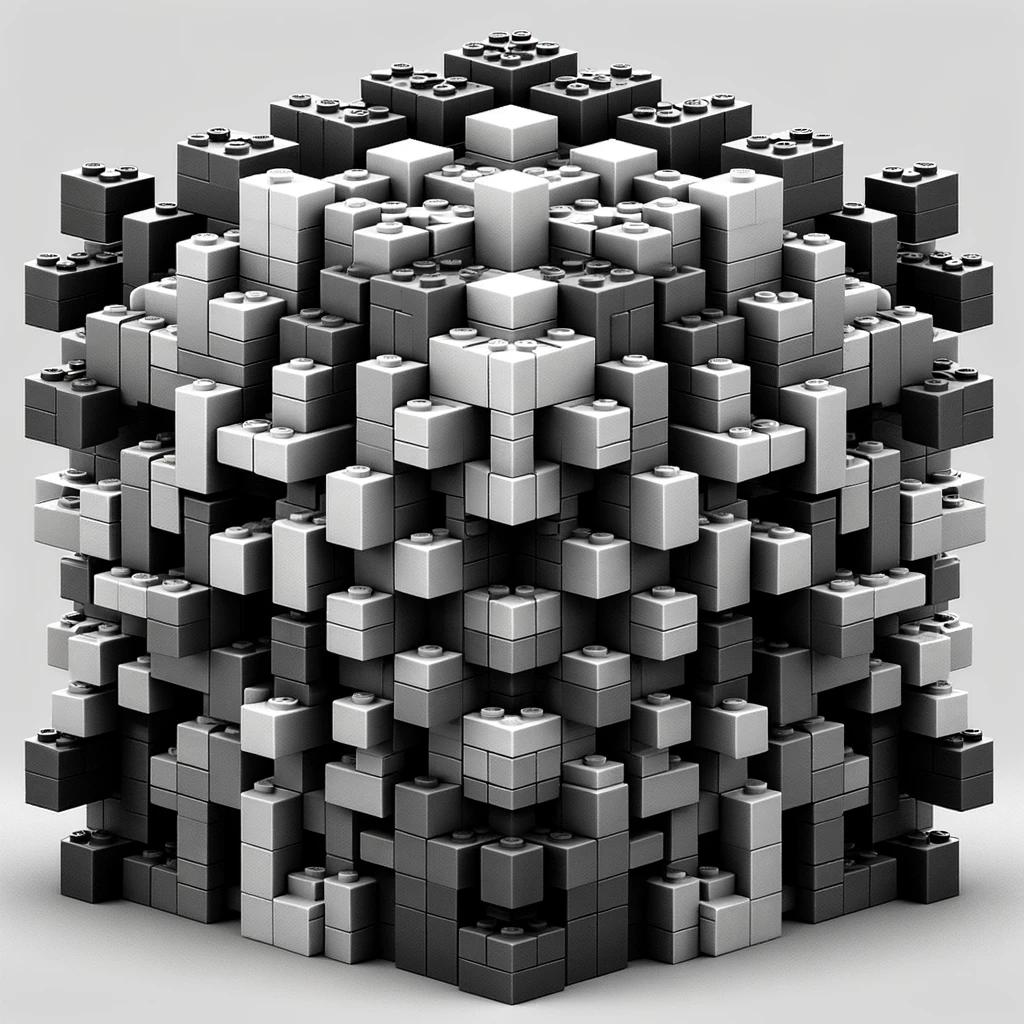
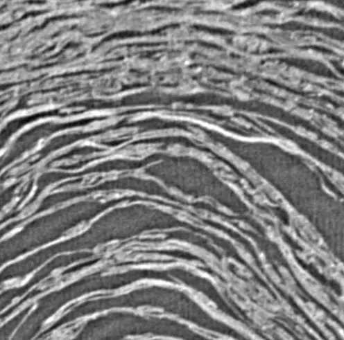
The right image in Figure 1 displays the view of a section of the volumetric image. Imagine cutting the volume in subvolumes. Take one and look at it from above. Every block composing the subvolume (called voxels) will look like a colored square. That is the color of the pixel in the image.
Node placement
To perform node placement we have to detect all the blocks composing the inner surface of the sheet, and forget about the rest. This accounts to creating a mask where non-edge blocks are flagged with 0s and edge blocks are flagged with 1s. In layman's terms, color in black all the non-edge voxels, and in white the edge voxels.
Surface detection
What Thaumato Anakalyptor does is exactly this: it performs surface detection in 3D by convolving the volumetric image with a 3D Sobel Kernel.
In simpler terms, it computes a discrete approximation of the 3D color gradient. Then, driven by the intuition that the greatest variation in color will be on an edge, it filters out all the voxels for which the magnitude of a gradient is small (below a given threshold).
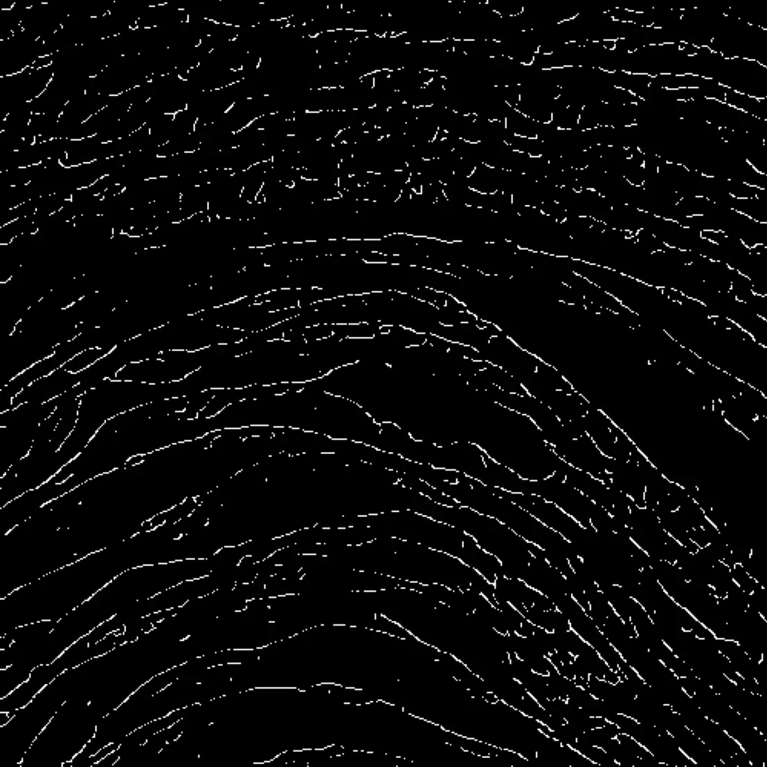
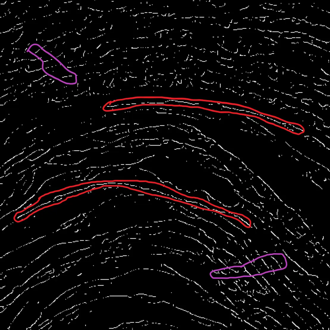
At the same time, considering for every voxel a vector that points towards the umbilicus of the scroll (the pole of rotation), and taking the dot product between this vector and the gradient computed just before, one can filter out as well all the voxels that are on the face of the sheet that don't look towards the center. In Figure 2 we display a sagittal view of the mask for the subvolume showed in Figure 1. The image was obtained with a modified version of Thaumato Anakalyptor.
Point Cloud Extraction
Unfortunately, our net still cannot get in. Instead of having grayscale LEGO blocks, we now have black/white LEGO blocks. The colors of the blocks changed, but we are still talking about a dense volume. In order for the net to get in we need to create some empty space. This means performing a change of representation. Instead of dealing with LEGO blocks located at positions (i,j,k) on a tridimensional grid, we will transform the blocks into infinitesimal points located at positions (x,y,z) in Euclidean space.
At the same time, we throw away all the black blocks (that now are points), and we keep just the white ones (those that lie on the sheet surface).
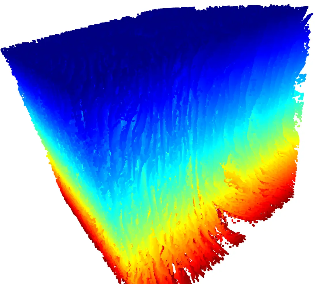
We extracted what is called a point cloud. In Figure 3 we show a point cloud obtained with a modified version of Thaumato Anakalyptor, colors are added just for the purpose of display, since the cloud is very dense. As you may notice, the subvolume looks like a jungle of points that kind of align in parallel sheets. Remember to keep a copy of the computed gradients since they will be eventually needed in the next steps.
Exploiting the created empty space, our fisherman net can now enter the scroll. Every node of the fisherman's net will be placed on a point in the point cloud. But how exactly? We want the net to overlay a contiguous patch of surface, without connecting parallel sheets. This problem will be addressed in the next section.
Connectivity establishment
We now have a cloud of points, and it's a mess! In order to fish a single, continguous patch of a sheet, we first have to identify adjacent parts of the sheets, dispatching every point in its proper neighborhood.
Segmentation
We don't want to select points that lie on parallel surfaces, since this would mean to identify as contiguous points that are not really contiguous in the scroll! We diplay the nature of this problem in the left part of Figure 4, where correctly grouped points are circled in red, and incorrectly grouped points are circled in purple.
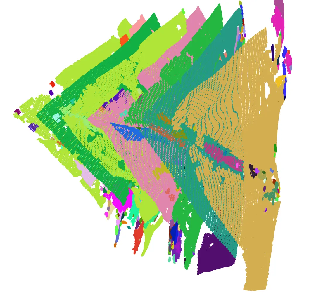
Thaumato Anakalyptor performs this operation with Mask3D 2, a Deep Neural Network specifically trained for the purpose.
The results should look somewhat like the right part of Figure 4 (that represents a different subvolume, less densely packed). The algorithm segments point clouds in contiguous patches of sheet.
Unfortunately, we have to face two unexpected problems:
- the algorithm creates patches with holes and in the holes there are other smaller patches;
- the area of these patches is too small.
Thaumato Anakalyptor tackles this issue with stitching.
Stitching
Stitching is an extension of the point cloud segmentation problem addressed in the previous step, but on patches rather than points.
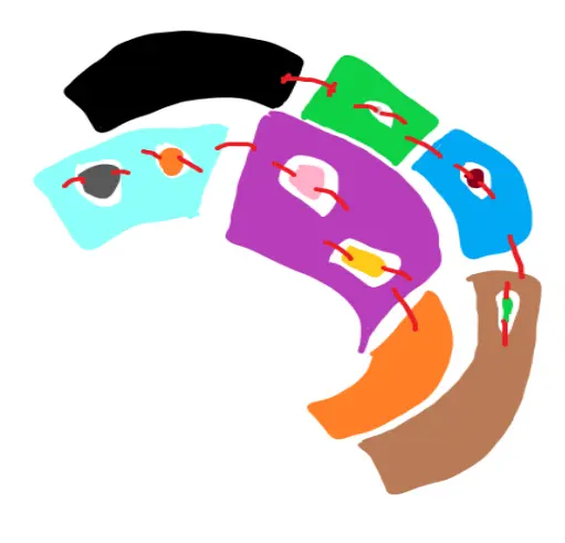
In Figure 5 different patches have different colors and patches that are stitched together are linked with red arcs. In the end, all the patches that are stitched together will form a segment, hopefully big enough to read on it some columns of text with ink detection models. It is worth saying that the segmentation performed by Thaumato Anakalyptor generates overlapping patches. The patch overlap is exploited during the stitching process.
Thaumato Anakalyptor performs stitching in a sort of Monte Carlo fashion. It first builds an uncertainty graph where nodes of this graph are patches and edges are weighted by the amount of overlap between patches. Many random walks are launched of the graph to build a subgraph (to select a cover of nodes/patches). The covers that selected the edges with the maximal overlap are chosen as final segments.
Mesh reconstruction
Now that we have a few big patches, represented as groups of point clouds made of contiguous points on the surface of the sheet, we can select one, and perform mesh reconstruction.
This means finally to establish a connectivity relationship between points: to decide which nodes that are connected in the fisherman net are connected in the point cloud as well. In layman's term, we find a way to connect points with edges!
Surface reconstruction can be performed with several algorithms, such as Poisson Surface Reconstruction 3 (that leverages both the positions and the normals to the points, i.e. the gradients that we computed in the previous steps) and Delaunay's triangulation 4. Thaumato Anakalyptor uses a mixture of both.
If instead of working on subvolumes we work on the full volume of the scroll, we can envisage ending up with a large contiguous mesh that is wrapped several times around the umbilicus. This is what Thaumato Anakalyptor can do, visualized in Figure 6.
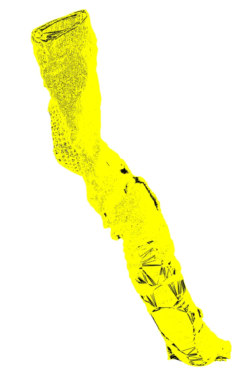
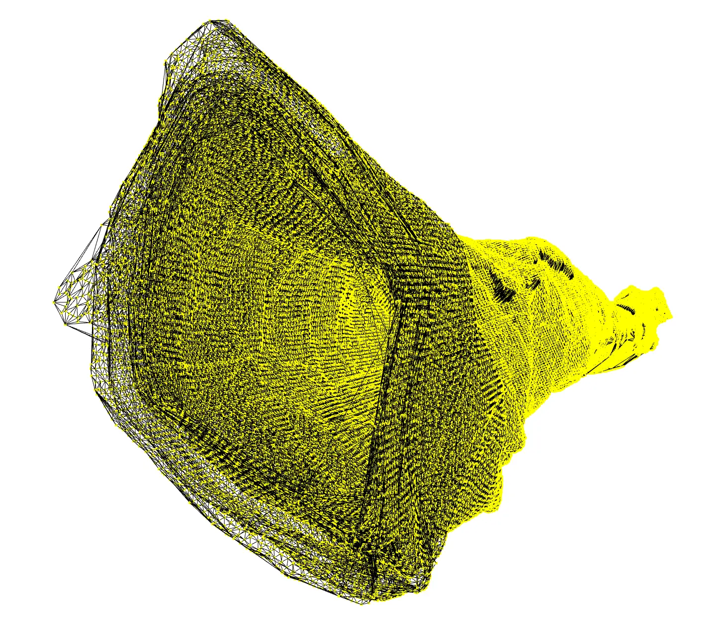
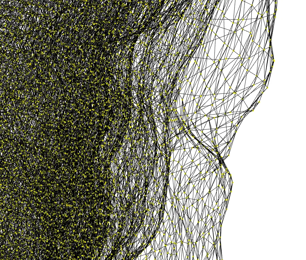
In Figure 6, the vertices of the mesh are shown in yellow and the edges connecting them in black. It is worth noting from the zoomed-in view that nearby points are connected by edges and form a triangular mesh.
Congratulations! You automatically fished the scroll, or a subpart of it!
Further steps
In this extra section we describe how from a triangular mesh we can obtain the 2D image of a sheet. This process involves two main steps: flattening and rendering.
Flattening
Now that we have a mesh, we must compute a 3D->2D map to obtain a UV (two-dimensional) parametrization for its vertices. This is a fancy way to say that you have to flatten the mesh. After all, our purpose is to eventually read the ink on a flat image.
A community fork 5, recently merged to Thaumato Anakalyptor, implements an algorithm called SLIM 6 that aims to find a map that minimizes an isometric distortion energy. This means that all the points that are equidistant in 3D will be mapped as equidistant as possible in 2D.
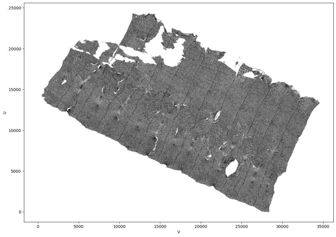
The vertices of the mesh shown in Figure 6 are displayed using the obtained UV parametrization in Figure 7.
The mesh, along with its UV parametrization, are finally saved in a .obj file.
Rendering
It is extremely important that the obtained UV coordinates are still real numbers. This means that between points there is a lot of empty space! In order to go back to a "pixel-style" representation, we have to convert the plot in Figure 7 to a pixelized image. Notice that in Figure 7 we displayed axes with ticks, this was not a mistake.
Per-pixel-map and layers
For every integer couple (x,y) in the figure we insert a new point. These coordinates (x,y) will be the integers' positions (i,j) of pixels in the rendered image. Eventually, we will end up with a number of points way higher than that of the vertices of the mesh. We will identify in which triangle of the triangular mesh (in 2D) these points fall and compute their barycentric coordinates: three coefficients that allow to define the position of every point in a triangle as a linear combination of the positions of the vertices. In Figure 8 we show a red point whose position will be 0.2 * vertex1 + 0.3 vertex2 + 0.5 vertex3.
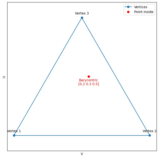
Exploiting the barycentric coordinates, we can then map back every additional point that we inserted in the UV map to its alleged position in 3D space.
This step is called obtaining a per-pixel-map and it's performed in Thaumato Anakalyptor using a recently merged community fork 7.
Why do we need the 3D positions of the new points? Remember that during the first step, Node Placement, we totally forgot about the density of the material obtained via the CT scan (its original color) and started working on a black and white mask, that later became a point cloud, and so on. All the colors displayed in Figures 3-7 were only for representation purposes.
Now we need to recover that information, and to do so we need to know the 3D position of every new point that is going to become a pixel of our rendered image. Unfortunately, the map from integer 2D positions to 3D points will result in points with non-integer positions. What does it mean? After all, the original voxels (Figure 1) only have integer positions. What "color" will these new points/pixels then have?
We are going to compute the color of the new points by trilinear interpolation with their closest ones in the volume.
This will allow us to obtain images with a smooth varying color. The segment from Figure 7 rendered as a 2D image is displayed in Figure 9.
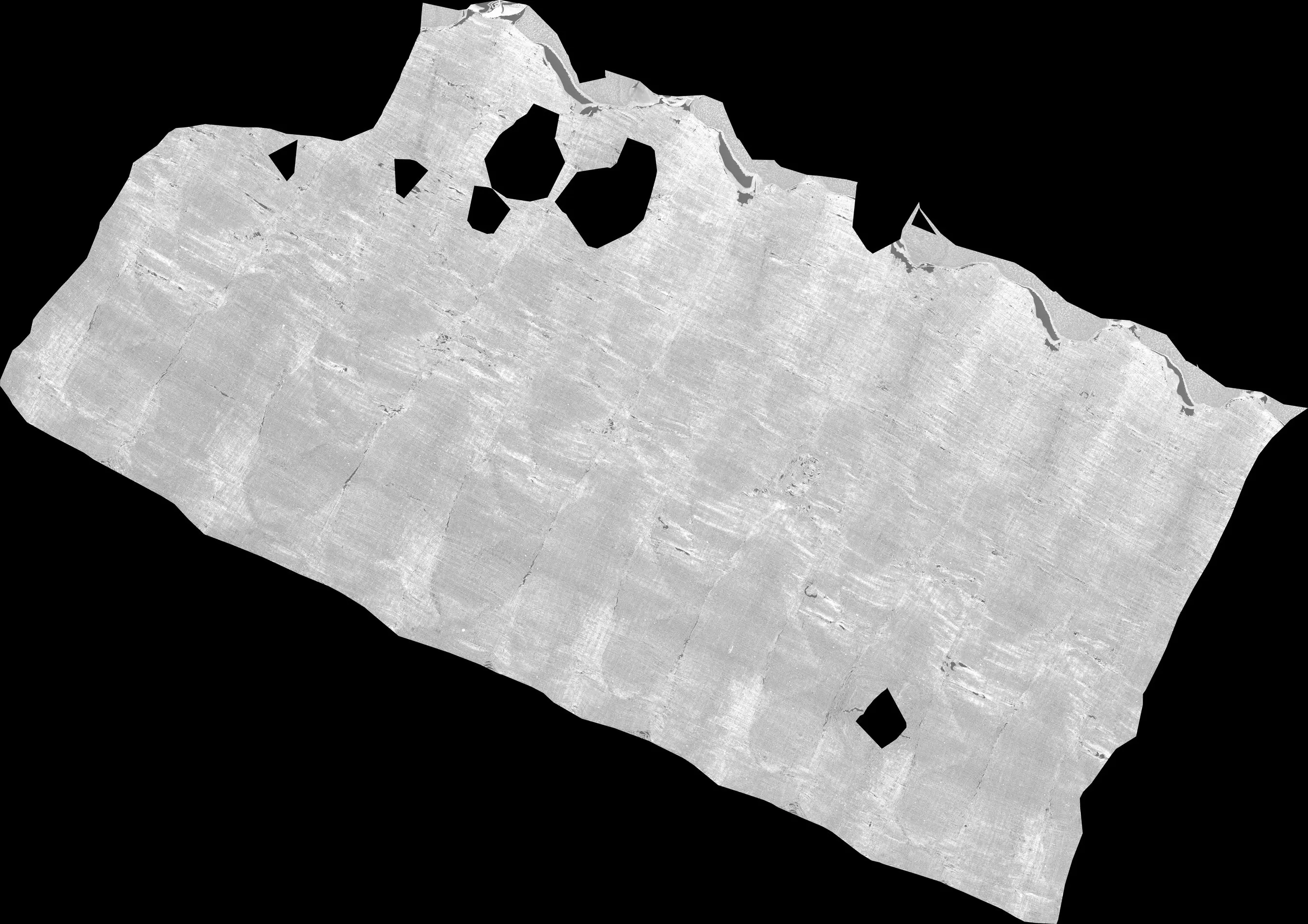
We forget to mention that since ink prediction is performed not on a single layer, but in what is called a surface volume, that is a stack of surfaces parallel to the surface we obtained along this pipeline, we need to store and transform as well the values of the normals to the surface at each point. We already computed them for the vertices of the mesh, so we only need to compute the ones for the new points using barycentric coordinates.
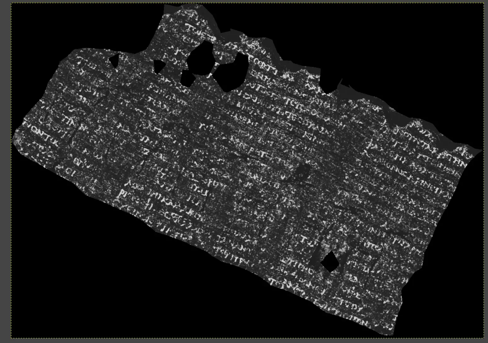
In Figure 10 we show the ink prediction from the Phase 1 Grand Prize winning model 8 on the stack of rendered layers obtained from the segment displayed in Figure 7 - the composite image is shown in Figure 9.
Additional notes
Please notice that every single one of the previously mentioned steps can be improved, both in terms of mesh generation quality and computational efficiency.
For further information on Thaumato Anakalyptor and its roadmap, please read its official Technical Report.
References
Footnotes
-
Schilliger et al. (2023). Thaumato Anakalyptor. Retrieved from https://github.com/schillij95/ThaumatoAnakalyptor ↩
-
Schult et al. (2023). Mask3D: Mask Transformer for 3D Semantic Instance Segmentation. Paper presented at the International Conference on Robotics and Automation (ICRA). ↩
-
Kazhdan et al. (2006). Poisson Surface Reconstruction. In Proceedings of the Eurographics Symposium on Geometry Processing. ↩
-
Delaunay, B. (1934). Sur la sphère vide. Bulletin de l'Académie des Sciences de l'URSS, Classe des Sciences Mathématiques et Naturelles, 6, 793-800. ↩
-
Angelotti, G. (2024). slim-flatboi. Retrieved from https://github.com/giorgioangel/slim-flatboi and https://github.com/schillij95/ThaumatoAnakalyptor/pull/2 ↩
-
Rabinovich et al. (2017). Scalable Locally Injective Mappings. ACM Transactions on Graphics (TOG), 36(4), 1. ↩
-
Angelotti, G. (2024). Democratizing rendering. Retrieved from https://github.com/schillij95/ThaumatoAnakalyptor/pull/6 ↩
-
Nader et al. (2023). Vesuvius Grandprize Winning Solution. Retrieved from https://github.com/younader/Vesuvius-Grandprize-Winner ↩