Tutorial: Segmentation and Flattening
This page has been archived and is no longer maintained. It describes an earlier generation of the Vesuvius Challenge pipeline — tools, data layouts, and results referenced here may have been superseded. See Open Problems for the current state of the pipeline and Prizes for what is open today.
This tutorial walks through a slice-based approach to segmentation, which is helpful background for learning about the task. This was used to generate the 2023 Grand Prize results. We are now working on more automated, 3D approaches to segmentation.
Please see the accompanying video tutorial for segmentation using Volume Cartographer here: https://www.youtube.com/watch?v=gdQmepxWhuY
As we saw in the "Scanning" tutorial, it’s quite hard to extract useful information out of a “word soup”, even when the ink is quite clear. For this tutorial we’ll show how to use virtual unwrapping to produce a flattened image which shows the content clearly.
Two key steps to virtually unwrapping a scroll or manuscript are segmenting a surface from inside the 3D volume and flattening that surface to 2D. The video below shows the idea quite well; or check out the full version (It was made by Dr. Seales’s son and daughter!). The red line during the reconstruction phase represents the surface that we want to virtually unwrap.
To perform segmentation, you have two choices of software: Khartes, and Volume Cartographer. Both of these choices have different strengths and weaknesses, but either can accomplish the task of accurate segmentation. Khartes relies on Volume Cartographer to perform the flattening portion of this guide. Thanks to @hari_seldon and @djosey of the segmentation team for their feedback and help with making this guide!
- Volume Cartographer
- Khartes
Strengths:
- Faster at creating larger segments
- tool-assisted annotation, requiring less clicking
- Entire pipeline in one application
- No shape limitation (lines can turn in on themselves, can be fully circular)
Weaknesses:
- Can only segment on the Z plane, which is a challenge in some areas
- No preview during segmentation
- Relatively high hardware requirements
Strengths:
- View z, x, and y planes and segment on any of them
- Interactive full scroll movement through ome-zarr
- Minimal hardware requirements
- Live view of segmentation results, enabling very high accuracy
Weaknesses:
- Is limited to creating segments that do not contain lines that turn back towards their origin, in essence limiting you to half circles at most. This can be severely limiting in some regions that have severe warping, and its hard to tell when you begin if a sheet will do this eventually.
- Requires much more manual clicking than VC
- Requires VC in some parts of the rendering / flattening pipeline
Khartes is written by @khartes_chuck and has extensive documentation on github located here.
This guide will focus on Volume Cartographer, a virtual unwrapping toolkit built by EduceLab’s Seth Parker. Volume Cartographer is designed to create meshes along surfaces of a manuscript (e.g. pages or scroll wraps) and then sample the voxels around these meshes to create a 2D image of the manuscript's contents. Volume Cartographer includes many tools and utilities. In this tutorial we’ll be looking at the main VC GUI as well as the vc_render tool. Volume Cartographer screenshots and recordings below are © EduceLab/University of Kentucky.
The segmentation team uses a custom version of Volume Cartographer, initially forked by @RICHI and further enhanced by @spacegaier. These versions include significant improvements, such as Optical Flow Segmentation (OFS), substantial performance increases, ui improvements, and many other changes. The latest fork, maintained by @spacegaier, is available here: https://github.com/spacegaier/volume-cartographer.
This guide uses this same version of VC. If you use a different version this guide will vary significantly from your experience, so it is highly recommended to use this version.
Installing Volume Cartographer
To begin, let's install Volume Cartographer:
- Windows
- macOS (using Homebrew)
- macOS (using Docker)
- Linux
- Build from source
- Install the VcXsrv Windows X Server or a similar X Server (if you use the Chocolatey package manager:
choco install vcxsrv). - Run “XLaunch” from the Start Menu, or from “C:\Program Files\VcXsrv\xlaunch.exe”.
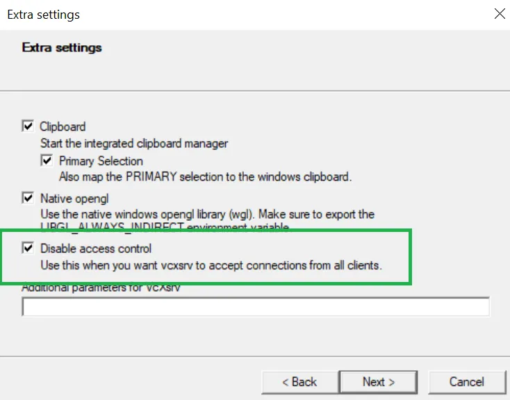
- Use the default settings, except:
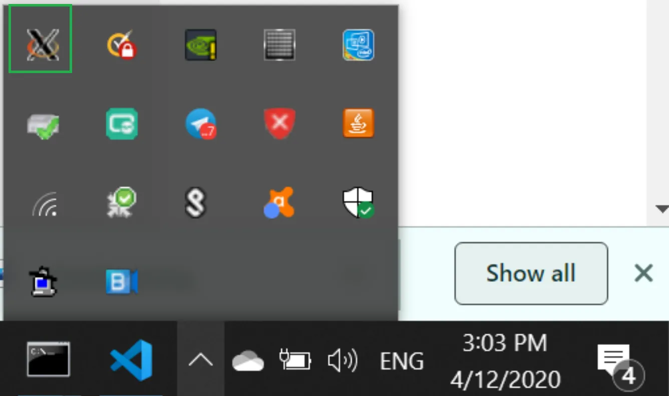
- Check that the X Server is running in the tray:
- Install Docker Desktop.
- Pull the latest Docker image by running:
docker pull ghcr.io/spacegaier/volume-cartographer:edge
Note: this does not install the fork of Volume Cartographer mentioned above.
Install Homebrew. Run brew install --no-quarantine educelab/casks/volume-cartographer.
- The GUI app will be installed to
/Applications/VC.app. - The command line tools are installed to
\$(brew --prefix)/binand should be available in the terminal immediately (e.g.vc_packager) — if not, make sure you haveeval \$(/opt/homebrew/bin/brew shellenv)in your shell profile and restart your terminal.
- Install XQuartz: https://www.xquartz.org/
- Log out and back into macOS.
- Launch XQuartz. Under the XQuartz menu, select “Preferences”.
- Go to the “Security” tab and ensure “Allow connections from network clients” is checked.
- Quit XQuartz and restart it.
- Install Docker Desktop.
- Pull the latest Docker image by running:
docker pull ghcr.io/spacegaier/volume-cartographer:edge
- Then run:
xhost +localhost
- We assume that you’re running the X Window System (if you’re unsure, you probably do).
- First, install Docker. Do not use Snap to install it.
- Pull the latest Docker image by running:
docker pull ghcr.io/spacegaier/volume-cartographer:edge
- Then run:
xhost +local:docker
- First, install basic build dependencies like
build-essential,cmake, and Qt6. - Then:
# Recursive clone, so we get the vc-deps repo, which contains dependencies.
git clone --recursive https://github.com/spacegaier/volume-cartographer.git

# Build vc-deps.
cd volume-cartographer/vc-deps
mkdir build && cd build
cmake -DCMAKE_BUILD_TYPE=Release ..
make -j

# Build main app.
cd ../..
mkdir build && cd build
cmake -DVC_PREBUILT_LIBS=ON -DCMAKE_BUILD_TYPE=Release ..
make -j

# Install, or skip this and refer directly to the executables in build/bin.
make install
Gathering data
Now let's gather our scroll data and setup our folders...
We're going to start with Scroll 1 (PHerc. Paris 4) as this is the scroll that the 2023 Grand Prize segments were from, and is also the easiest of the current scrolls to segment. VC requires all of the folders listed under the PHercParis4.volpkg, in addition to the config.json and meta.json files.
This is the recommended structure for the full_scrolls folder (with a full example given for Scroll1):
full_scrolls/
  ├── Scroll1/
  │   └── PHercParis4.volpkg/
  │       ├── volumes/
  │       │   └── 20230205180739/
  │       │       ├── 00000.tif
  │       │       ├── .
  │       │       ├── .
  │       │       ├── 14375.tif
  │       │       └── meta.json
  │       ├── paths
  │       ├── renders
  │       ├── working
  │       └── config.json
  ├── Scroll2
  │   └── PHercParis3.volpkg/
  ├── Scroll3
  │   └── PHerc332.volpkg/
  └── Scroll4
      └── PHerc1667.volpkg/
And this is the recommended structure for your new_segments folder:
new_segments/
  ├── Scroll1
  ├── Scroll2
  ├── Scroll3
  ├── Scroll4
  └── run_vc.sh
To download the data, first navigate to the /volumes/20230205180739 directory. You can also place the files in /volumes/20230205180739 after they are downloaded.
Use this rclone command to download all of the Scroll 1 volumes quickly:
rclone copy :http:/full-scrolls/Scroll1/PHercParis4.volpkg/volumes/20230205180739/ . --http-url https://dl.ash2txt.org/ --progress --size-only
If you wish to begin with a smaller portion of Scroll 1, rather than the entire scroll, you can download 1cm of scan data from the center using:
for i in `seq 6000 7250`; do wget http://dl.ash2txt.org/full-scrolls/Scroll1/PHercParis4.volpkg/volumes/20230205180739/0\$i.tif; done
Be sure to have the config.json file at the root of the .volpkg directory, and the meta.json file in the volumes directory so that VC can work with it.
More information can be found at the Vesuvius Data Download Repo.
Running the Volume Cartographer GUI
We will use the main VC GUI app to perform segmentation: finding a surface of papyrus and exporting it as a 3D mesh.
This guide was written using Linux. Most of the commands are similar, but you may need to remove 'sudo' from the front of the commands depending on your operating system.
The -v switch used below is mapping a local path (or volume) to the Docker container. To check if your paths have been created properly you can run the Docker container and initiate a list command by typing:
docker run -v \path\to\full_scrolls\:/full_scrolls ghcr.io/spacegaier/volume-cartographer:edge ls
If you see your scroll folders, you’ve probably mapped this correctly.
Open a terminal and run (replacing the paths with your folder paths to the same folders):
sudo docker run -v /path/to/new_segments/:/new_segments -v /path/to/full_scrolls/:/full_scrolls -e DISPLAY -v /tmp/.X11-unix:/tmp/.X11-unix ghcr.io/spacegaier/volume-cartographer:edge VC
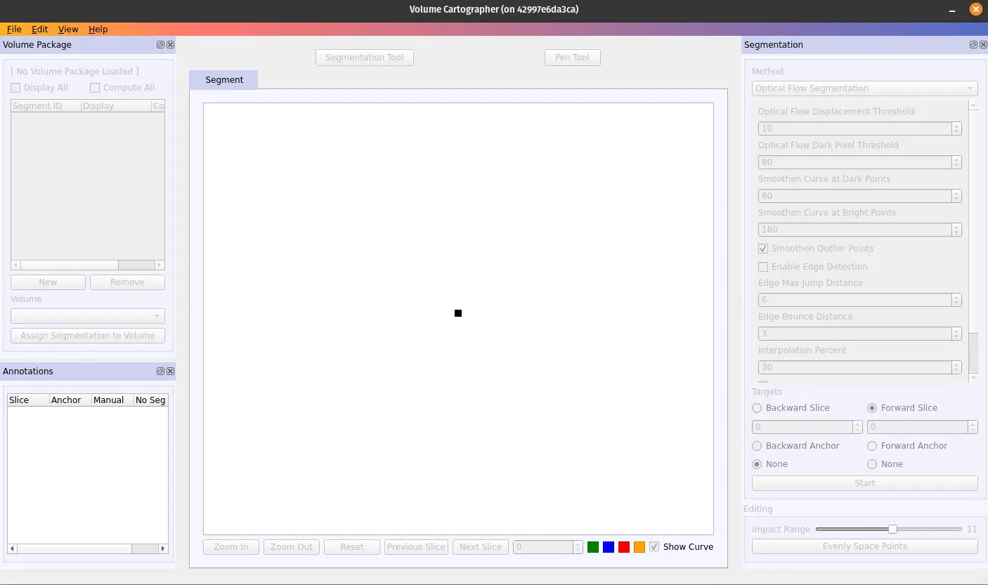
Let's take a moment to get oriented before continuing:
- In the top left are the current segmentations, or paths, in the current volume package (from here on referred to as a volpkg) along with the file, edit, help and view buttons.
- In the bottom left are the current segmentation runs and anchor information for the currently selected segment id.
- On the right are your OFS Segmentation settings.
- Located at the bottom is some navigation information. The primary number useful to you here will be the current slice number.
Navigating a .volpkg
Now that we’ve oriented ourselves with the UI, let's open our .volpkg...
- Open a .volpkg by clicking file, then open .volpkg, and select the .volpkg for the volume you wish to segment on, ensuring you select the .volpkg folder, and not one of the subfolders. Click choose, and the volume will open at slice 0.
- Practice scrolling through the volume, using shift+scroll wheel to move up and down through slice layers, and ctrl+scroll wheel to zoom in and out. You can right click and drag to pan around the slice. Move through the layers until you find an area of the sheet that looks “easy” to segment. An ideal area has spacing on the inside face towards the center of the scroll, and maintains this spacing as you scroll through the layers for a time. You can increase the amount of slices you move through with the scroll wheel by pressing Q and E. The small number that shows up next to your cursor is the number of slices skipped each “click” of the scroll wheel.
- Look now to the top left in the segments window; our VC shows some segmentations in the segmentation window, but yours at this point will be blank.
Creating a segment
We will now create our first segment.
Click "New" in the Volume Package segmentation window on the top left to create a new segment path. Ensure "Display" and "Compute" are both checked.
Click “Pen Tool”, and place points along the sheet by left clicking, placing as many points as necessary to keep the line on the surface of the sheet. Note that you cannot undo or delete points here. This part does not need to be particularly accurate, as you’ll be able to fix it in the next step much easier. When you are happy with the length of the line, click pen tool once again to exit the pen tool.
You’ll notice now that the purple line becomes a series of points. This is your “segmentation line”. It is from this line that VC will create your final flattened surface volume. Ideally, you want this to be on the inside face of the sheet, as this is where we expect to find ink.
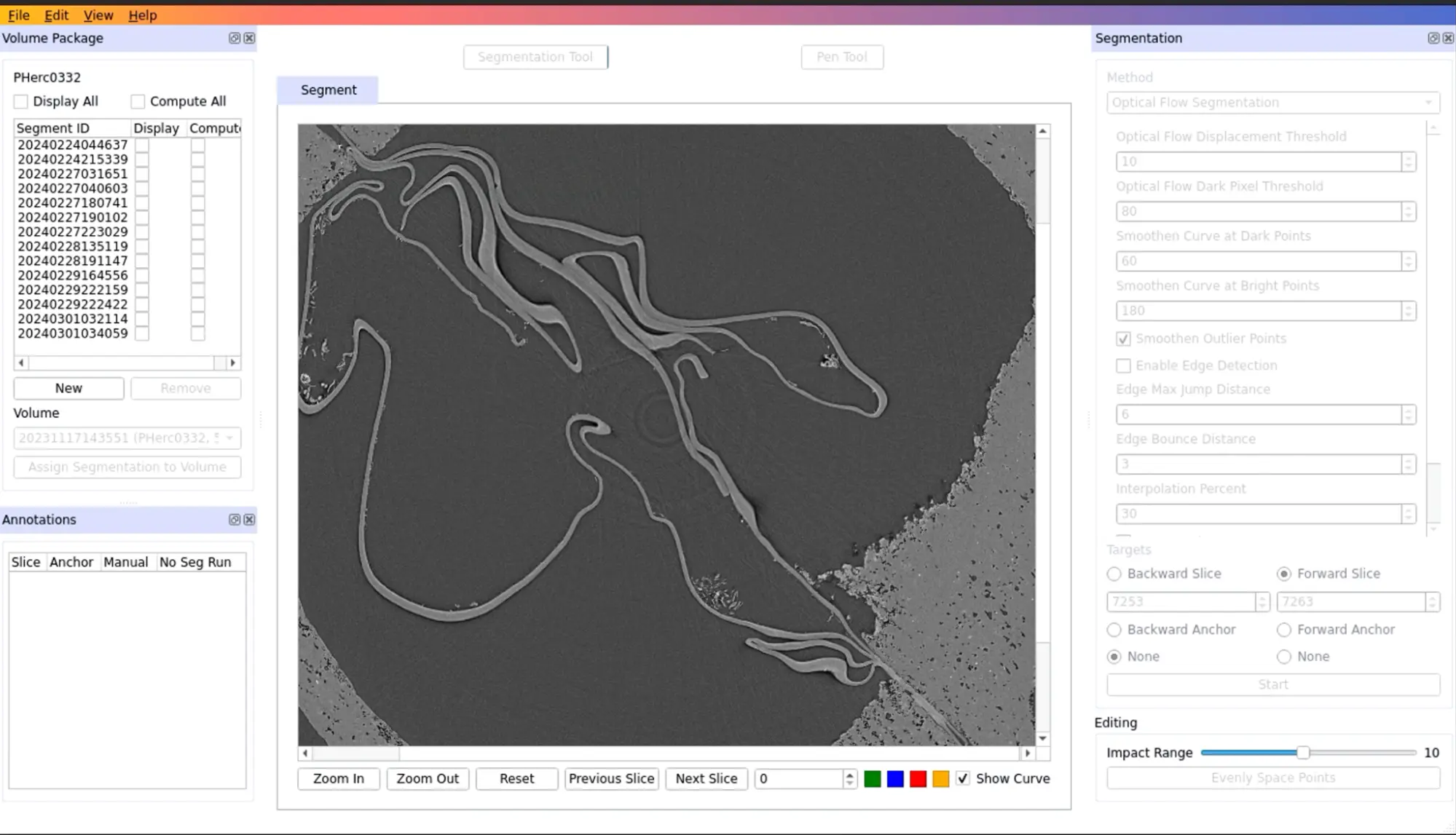
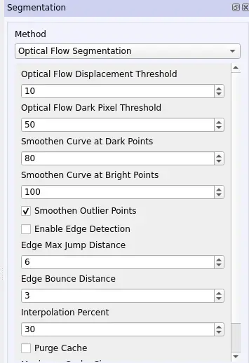
Now, click “Segmentation Tool” (You can also enter the segmentation tool by pressing 'T'). Let’s configure our Segmentation settings in the right box to match the ones in this image. The primary parameter you could modify here and see if you have any improvement is 'smoothen curve at bright points'.
If at this point your segmentation line is off the sheet, you can manipulate it in a few ways. The primary method for manipulating this line is to “snap” it to a point, by clicking. VC will take the X nearest points to the cursor (where X is the input range setting located in the bottom right, also in/decreased by hitting A and D respectively) and snap them to the cursor. You can also click and drag the line itself. Play around with this for a bit before continuing. In addition to just panning along the line with right click, you can press R+Scroll Wheel to follow the segmentation line automatically. This is also mapped to the front and back side mouse buttons, if you have them.
Once you are happy with the location of the line, ensure your slice and anchor settings are correct. If you’re going “up” in the volume, you want forward slice and backward anchor, and conversely if you're going “down” in the volume, you want a forward anchor and “backward slice”. The number in the forward or backward slice is the number the segmentation run will finish at. It is recommended to start low here, between 30 and 50, and depending on how far the line diverges from the sheet, you can increase from there. In areas of particularly damaged papyrus values as low as 10 can be required.
Click “Start” to begin the segmentation run.
After a short period of time VC will drop you off at the slice indicated by your previous forward or backward slice setting. Your line of points will now be colored red, and may have wandered slightly from the sheet. VC has attempted to “follow” the sheet from your annotation (or anchor) line to the slice indicated in your forward slice setting. From here, click “segmentation tool” again, and then manipulate the line back onto the sheet. You’ll notice lines you have modified turn yellow, where ones you have not remain red. Pan through the layers a bit if you are having a hard time following the sheet, as it's easier to follow “in motion”. Press space to hide the line if it helps you see.
You can press T at any time within the segmentation tool to return to the slice you began the segmentation on.
After you’ve guided the line along the sheet, hit “Start” again, and repeat the process. This is the general workflow for segments of any size, from the GP winners at over 100cm^2 to the smallest segments. Conceptually, it works something like this:
Be sure to save it using “File > Save volpkg”. You can keep segmenting for a bit here to get the hang of VC, but keep the size manageable for your first few segments until you get more familiar.
The process completed during this step looks like this in 3D. We've identified the sheet surface, but still would have a hard time finding ink on a single voxel sheet that is still wrapped in the scroll. In the video below, the sheet is on the visible outside, but most of our segments are completely surrounded by additional sheets.
Flattening and texturing
Ok, we've got a line...Now what?
In order to see the content on the surface of our segment, we need to flatten and texture the segment. These steps can be run individually, but it’s highly suggested to use the following process so that you end up with the same format and files as the official segmentations.
Let's create a bash script to combine a number of different VC apps into one single command:
- Open a basic text editor (ex: Notepad)
- Copy this code block into the editor
#!/bin/bash

# Set environment variables
export SEGMENT=20240227040603 #change to the segment number you've created
export SCROLL="Scroll1/PHercParis4.volpkg" #change to whatever scroll you are currently working in


# Navigate to the segment folder, create a directory named after \$SEGMENT
cd \${SCROLL}
mkdir -p "\${SEGMENT}"
cd "\${SEGMENT}"

# Copy necessary files from the scroll folder to the current directory
cp "/full_scrolls/\${SCROLL}/paths/\${SEGMENT}/pointset.vcps" .
cp "/full_scrolls/\${SCROLL}/paths/\${SEGMENT}/meta.json" .
cp "/full_scrolls/\${SCROLL}/paths/\${SEGMENT}/pointset.vcano" .

# Convert and render pointset, then generate layers and calculate area
nice vc_convert_pointset -i pointset.vcps -o "\${SEGMENT}_points.obj"
nice vc_render -v "/full_scrolls/\${SCROLL}/" -s "\${SEGMENT}" -o "\${SEGMENT}.obj" --output-ppm "\${SEGMENT}.ppm" --intermediate-mesh "\${SEGMENT}_intermediate_mesh.obj" --save-graph 0 --orient-normals

mkdir -p layers
nice vc_layers_from_ppm -v "/full_scrolls/\${SCROLL}" -p "\${SEGMENT}.ppm" --output-dir layers/ -r 32 -f tif --cache-memory-limit 50G

vc_area "/full_scrolls/\${SCROLL}" \${SEGMENT} | grep cm | awk '{print \$2}' | tee area_cm2.txt

# Set author name
echo '<YourNameHere>' > author.txt
-
Modify the environment variables at the top of the script, the ones that begin with
export, and the author at the bottom. You'll want these values to reflect the scroll you're working in, the name of your segment, and who you'd like to list as the author. -
Name the script
run_vc.shand save it to the 'new_segments' directory
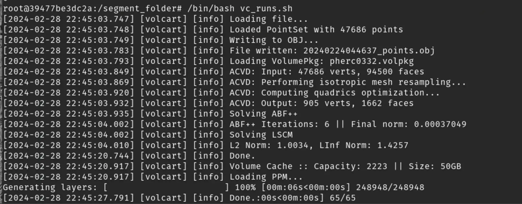
Once we have our script created and have the right values for the environment variables, we can now execute the flattening pipeline. Open a new terminal (not the one you have the GUI running in), and enter
sudo docker run -it -v /path/to/new_segments/:/new_segments -v /path/to/full_scrolls/:/full_scrolls -e DISPLAY -v /tmp/.X11-unix:/tmp/.X11-unix ghcr.io/spacegaier/volume-cartographer:edge VC
The terminal for the container should open. Enter the following lines:
cd /new_segments/
/bin/bash run_vc.sh
This command will render your points into a mesh, and then create the surface volume layers from it. This can take a long time depending on the size of your segment, but thankfully you will get some progress information on the console.
Congratulations! You've completed your first segment!
In the new_segments directory you set when you launched VC, you will now have a folder with the name of your new segment, and within that folder a folder called layers/, and a number of different files, the most important of which are detailed below. Much of this information was gathered from @Seth P. and @khartes_chuck on the discord:
-
layers/contains files numbered 00.tif to 64.tif (or 000.tif to 156.tif for 3.24um scans). These are slices of the surface volume, each of a thickness equal to the voxel size of the scroll you are currently segmenting, typically what we call “low res” are the 7.91um voxel spacing, and “high res” would be 3.24um voxel spacing. For a 7.91um volume, this means that each surface volume is 64 tifs * 7.91um, for about 506um thickness, or .506mm. -
<SegmentNumber>.objthis is a 3D image format that stores information about the geometry of a 3D model, such as vertex positions, texture maps, normals, and faces. This is a mesh created from the pointset created by your segmentation line and detailed further below. -
<SegmentNumber>.tifis a composite image of maximum intensity pixels from within the surface volume, it is also used for texturing in combination with the mtl file. -
<SegmentNumber>.mtlis a text file that contains information about the material, such as opacity, reflectivity, and points to the texture file (the tif in the previous line). -
<SegmentNumber>.ppmA simple way to think about this is to think of it as a super dense point cloud that for each voxel in the flattened volume contains a point representing the 3d location in the original volume that voxel came from, and some information about that point. A better explanation is that a .ppm is special case of an ordered pointset, where type = double and dim = 6. It is generated by flattening the segmented surface, discretizing the parameterization, and storing the corresponding 3D point and surface normal for each spot on the surface. Using slice notation, ppm[y, x, 0:3] stores the 3D point and ppm[y, x, 3:6] stores the surface normal. Because the surface does not fill the 2D array entirely, there is a *_mask.png file next to the PPM. It stores which pixels in the PPM have valid values. More info here: Volume Cartographer PPM file format (github.com) -
<SegmentNumber>_mask.pngas detailed in the ppm description, just denotes areas that do not contain information from the scroll data. -
<SegmentNumber>.vcpsthis is the pointset created by your segmentation line. A .vcps file stores lists or 2D arrays of N-dimensional, numerical vectors. It starts with a header as described, then the points are written in sequence, usually in binary and rarely in ASCII. The type field in the header tells you the fundamental C++ type stored. -
<SegmentNumber>.vcanocontains information about which points were manually moved, and their original locations. -
Author.txtcontains the name of the person who created it. -
Area_cm2.txtis simply the size of the segment in cm^2.
Outputs
So, what did we just do?
When looking for ink in the volume, we need to look at more than just the voxels that directly intersect the segment mesh we just created. We also need to look a little bit “above“ and “below“ the mesh, at the neighborhood of voxels that surround our segment. Conceptually, this neighborhood looks something like this (though this video is exaggerated):
To generate the composite .tif file, called <SegmentNumber>.tif, vc_render searched through this neighborhood, gathering the voxel intensities, and placed the results of that search in the flattened output image.
The ppm file that we generated contains a mapping between our flattened output image and the original 3D surface. With this file, we transformed the 3D neighborhood into a simplified surface volume. That process looks something like this:
The result of this process are the 65 tifs in the /layers/ directory. Each of these .tif images is a "slice" of the surface volume, with 32.tif ideally representing the middle, or the area directly on your segmentation line.
Ink detection
So, where's the ink?
By now you'll notice that, contrary to the ink in some scrolls, the ink in our scrolls is not readily detectable in your images.
The reason for this is that not all inks have the same radio-density. Some inks, like iron gall, show up quite clearly in CT scans because they absorb more x-rays than the papyrus on which they sit. This creates high contrast between the bright iron gall ink voxels and the less bright papyrus voxels. Carbon-based inks, on the other hand, have a very similar radio-density to papyrus and thus have low contrast when compared against the papyrus voxels. More often than not, the contrast is so low for carbon ink that it is very difficult to differentiate the ink from the papyrus when looking at the volume data with the naked eye.
Thankfully, as you'll learn in our next tutorial on “Ink Detection”, even very difficult to detect ink can still be found...