Tutorial: Ink Detection

Last updated: August 14, 2026

Content feeling overwhelming? Catch up by asking Philodemus.

Ink detection is the last step of the pipeline: taking the flattened surface of a papyrus sheet (segmented from the 3D X-ray scan) and identifying where the ink is, so that the text can be read.

This is where one of the core difficulties of the Herculaneum Papyri comes in: the carbon ink and the carbonized papyrus have almost the same density, so in an X-ray scan the ink is nearly invisible to the naked eye. The problem is easiest to see on a detached fragment, where the writing is exposed and we can photograph it directly: in a color photograph the letters are faint, in 1000 nm infrared they are crisp and legible, but in the X-ray CT scan the ink contrast almost completely disappears.

(a) Color photograph

(b) 1000 nm infrared

(c) X-ray CT

Three images of the same detached fragment (P.Herc. Paris 2 fr. 47). The writing is faint in visible light, sharp in infrared, and nearly gone in the X-ray. Source: Stephen Parsons, Hard-Hearted Scrolls.

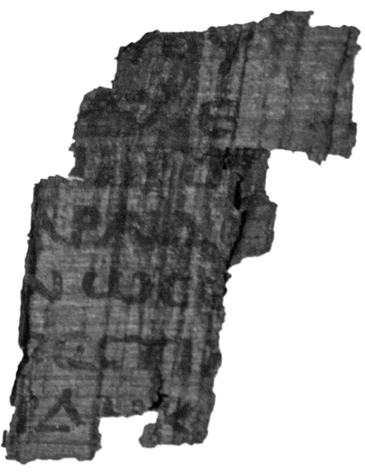
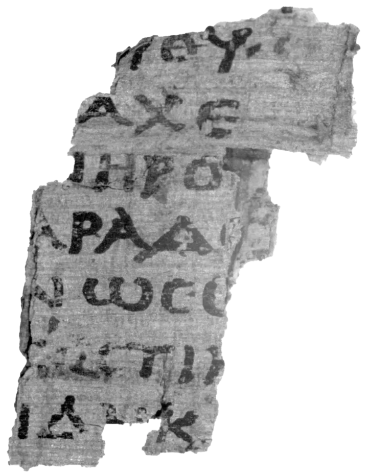
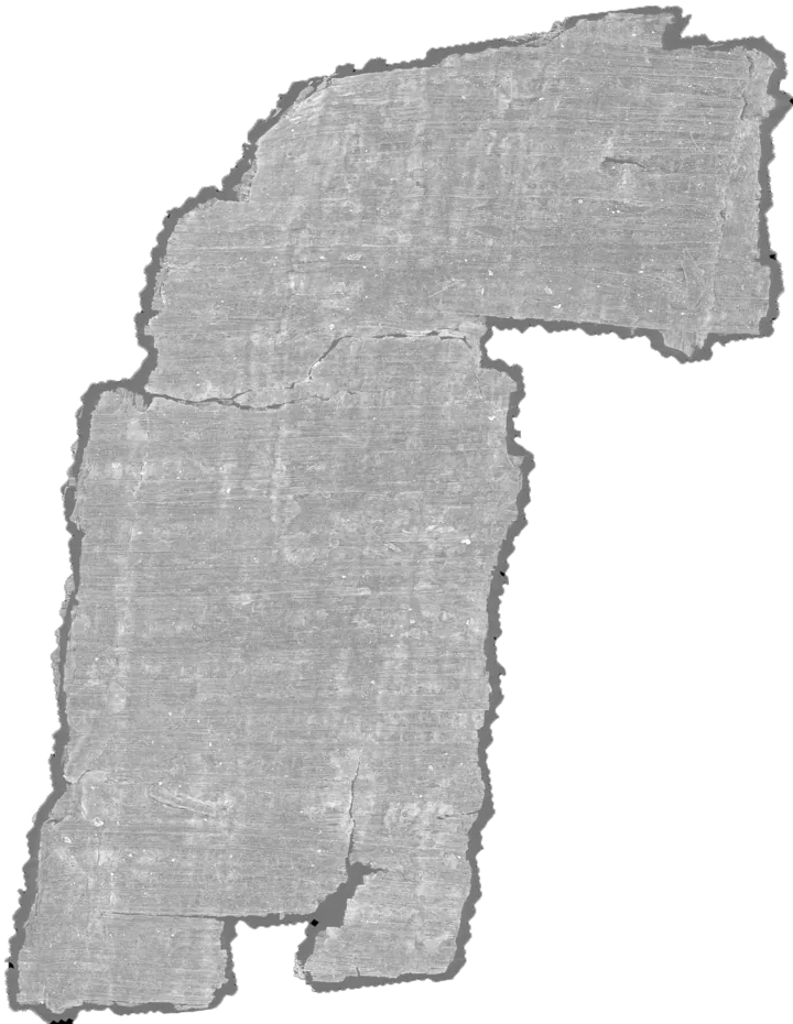
So why scan with X-rays at all? Because visible and infrared light can't see inside a rolled scroll — they don't penetrate the papyrus. X-ray CT does: it images the interior of an intact scroll at high resolution, but, as the fragment above shows, at the cost of the visible ink contrast. Ink detection exists to win that contrast back computationally.

Not all of that contrast is lost, though. What does the surviving signal look like? In PHerc. Paris 4 in particular, ink can sit as a thin layer on the papyrus surface, and on the flattened surface volume it often shows up as a crackle — a texture like cracked mud, raised slightly above the papyrus. Crackle is one of several surface-morphology cues that can betray ink; on other scrolls the signal is more subtle and heterogeneous, and may instead depend on fine texture, local roughness, deposits, or deformation.

The ink signal in the data: (a) a slice through the CT volume, (b) the same region with the ink segmented in red, and (c) a flattened surface volume where the crackle texture and the letter π are visible directly. Source: the PHerc. 1667 paper.

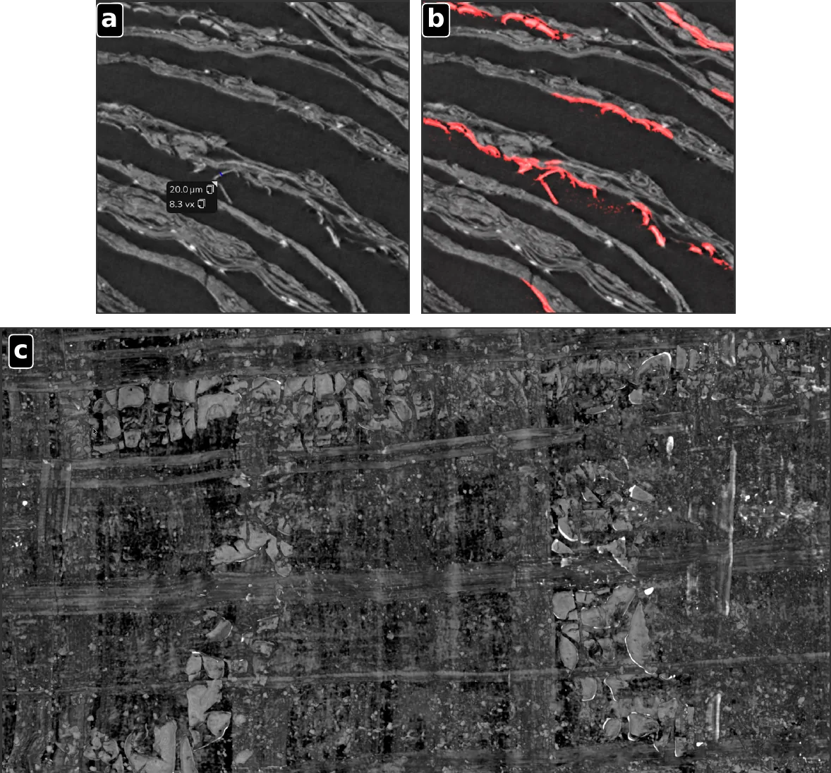
This crackle is what first revealed letters inside an intact scroll, spotted by eye in raw surface volumes. But it is the exception. Most scrolls show nothing so legible, so models trained on known ink learn to pick up traces the eye can't name. Several scrolls are still waiting for their first letters, and each is worth $50,000 in the open First Letters Prizes. Finding them takes a searching eye and a model's predictions. By the end of this tutorial you'll have both — and maybe you'll be the first person to read those words in 2,000 years.

How ink detection works

An ink detection model does signal recovery, not reading. The model looks at a small local patch of the surface volume (the stack of slices sampled around the papyrus surface) and predicts, for each pixel, the probability that there is ink at that location. Stitching these predictions together produces an image of the segment where the writing becomes visible to a human reader.

We train the model by picking a pixel in a binary label image, sampling a subvolume around the same coordinates from the surface volume, and backpropagating the known label to update the model weights:

We can then use the model to predict what a label image would have looked like, on data it has never seen:

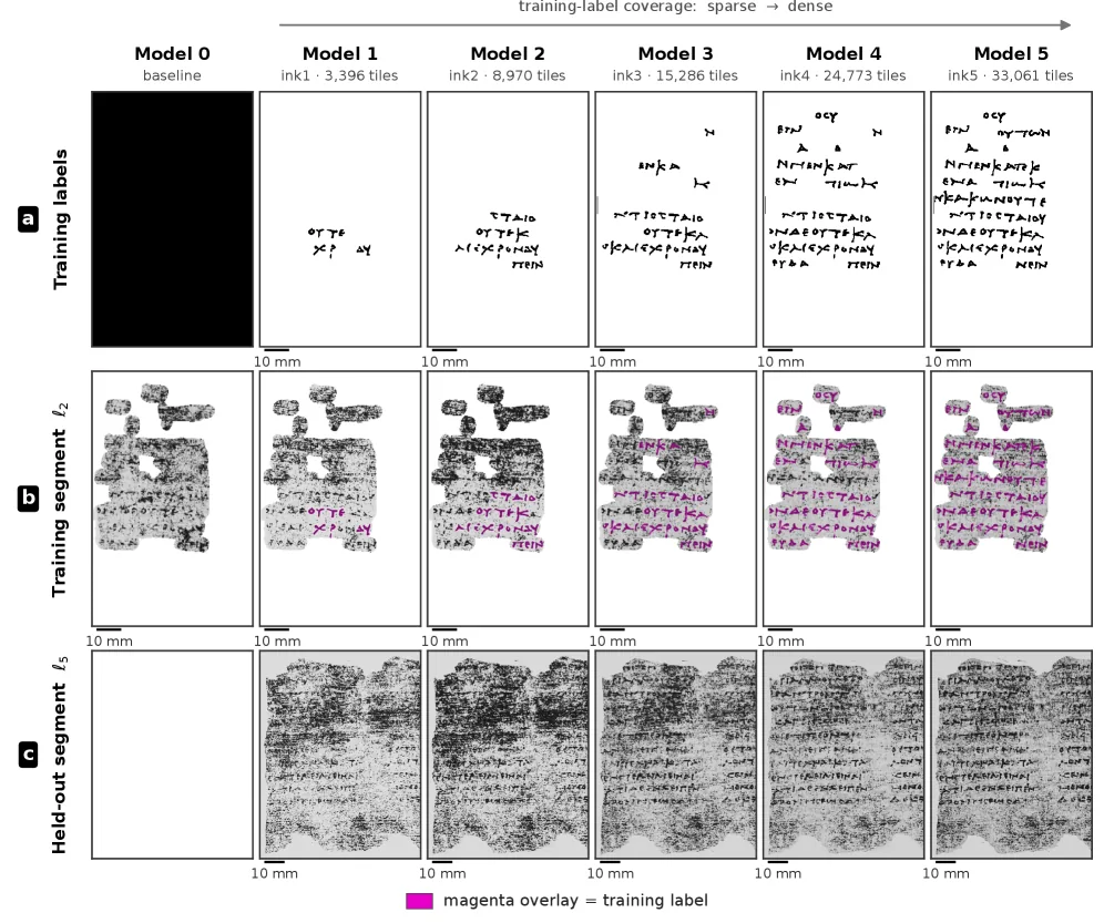
Where do the labels come from? The first ink labels came from detached fragments, where the exposed writing can be photographed in infrared and aligned with the surface volume. For the intact scrolls, labels are made iteratively: an existing model is run on a scroll segment, a human inspects the predictions, labels the regions where letter strokes are clearly visible, and the model is retrained on the enlarged dataset. Repeating this loop is how ink detection has improved from isolated letters to entire scrolls.

This process recently achieved the complete virtual unwrapping and reading of PHerc. 1667: the first Herculaneum scroll to be fully digitally unrolled and read without physical opening. The methods, including the labeling and validation methodology this tutorial is based on, are described in detail in the paper.

Because the labels come from model predictions, the process is designed to avoid reinforcing the model's own errors:

• The model only sees small local patches — smaller than a full letter — so it cannot learn to "draw" plausible letterforms.
• Labeling is conservative: only regions where strokes are clearly and repeatably visible get labeled.
• Validation regions are held out, so you can measure whether the model generalizes.
• Final readings are always reviewed by papyrologists. Machine output is never treated as a substitute for reading.

Now let's train a model. The rest of this tutorial is hands-on: you will set up the training pipeline, download a labeled dataset, train an ink detection model, and run inference on a scroll segment. It is written for Linux (Windows users are advised to use WSL2) and assumes an NVIDIA GPU with a working CUDA installation.

The dataset

The tutorial uses the ink-labels dataset, which lives in the scrollprize/datasets storage bucket on Hugging Face, organized by scroll. The full dataset is hundreds of GB, so the whole tutorial runs end-to-end on one segment of PHerc. Paris 4 (Scroll 1) — about 25 GB:

uvx --from huggingface_hub hf buckets sync \
  hf://buckets/scrollprize/datasets/ink/phercparis4/w00_20231016151002 \
  ./ink-dataset/phercparis4/w00_20231016151002

hf buckets sync works like rsync: re-running it resumes interrupted downloads and only transfers what changed. If you hit rate limits, create a free account, generate a read token under Settings → Access Tokens, and either run uvx --from huggingface_hub hf auth login once or set HF_TOKEN=hf_... in your environment.

Each segment is a folder in the layout the training pipeline expects, containing the surface geometry (.tifxyz), the surface volume, and the labels:

ink-dataset/phercparis4/
└── w00_20231016151002/
    ├── x.tif                                    # surface geometry: 3D coordinates
    ├── y.tif                                    #   of every surface pixel
    ├── z.tif
    ├── meta.json
    ├── w00_20231016151002.zarr                  # surface volume (image data)
    ├── w00_20231016151002_inklabels.zarr        # binary ink labels
    ├── w00_20231016151002_inklabels.tif         #   (and the editable TIFF original)
    ├── w00_20231016151002_supervision_mask.zarr # where the labels are trustworthy
    └── w00_20231016151002_supervision_mask.tif

The label files work together, and understanding them is the key to the whole pipeline:

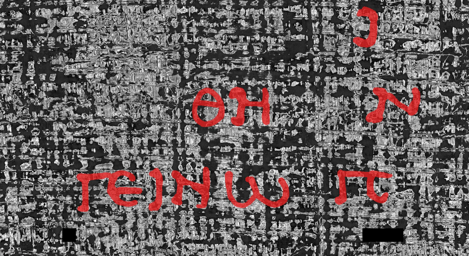
• Ink labels — a binary image aligned with the segment: white where there is ink, black where there is not.
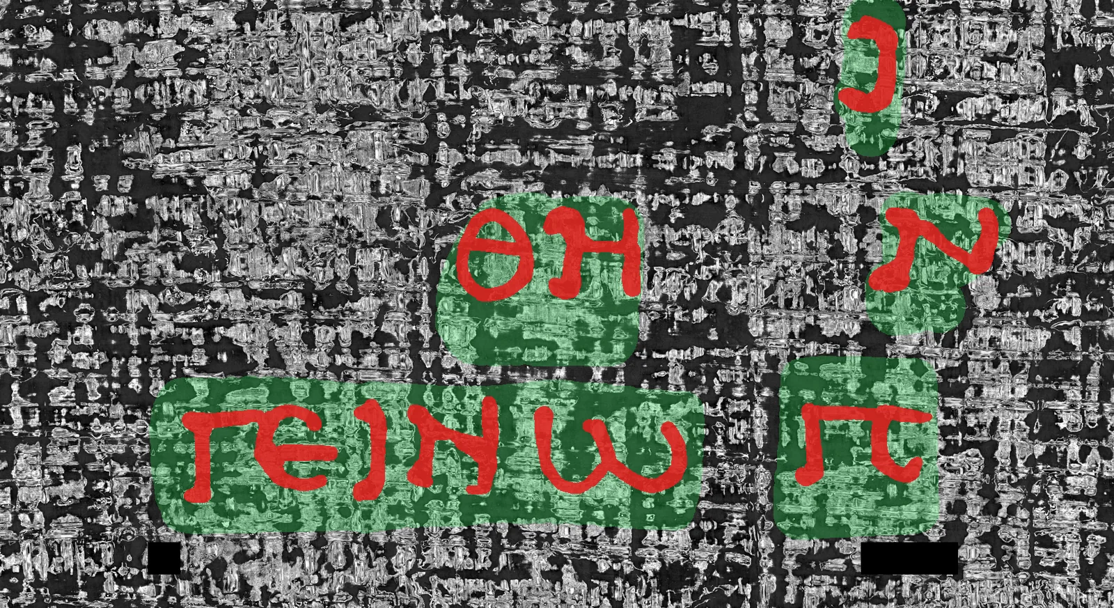
• Supervision mask — marks the regions where the labels can be trusted. Only pixels inside the supervision mask contribute to the training loss: white pixels there are positive (ink) examples, black pixels are negative (no ink) examples. Everything outside the mask is ignored, so unlabeled or ambiguous areas don't teach the model anything wrong.
• Validation mask — some segments also have a <segment>_validation_mask.zarr: a held-out region, labeled the same way as the rest, but excluded from training and used only to measure the model's accuracy. A segment without one (like the tutorial segment) still trains — you just get no validation metrics for it.

Here is what that looks like on a crop of the tutorial segment. First, the ink labels: strokes that a human labeler could clearly and repeatably see, painted on top of the surface volume:

A crop of the tutorial segment's surface volume with its ink labels overlaid in red

The supervision mask covers those strokes plus the clean papyrus around them. Those background pixels are the negative examples, and they matter just as much as the ink:

The supervision mask (green) marks where labels are trustworthy: both the ink strokes (red) and the unlabeled background inside the green region are used for training

info

The filename prefixes must exactly match the segment folder name: a segment folder named w00_20231016151002 must contain w00_20231016151002_inklabels.zarr, w00_20231016151002_supervision_mask.zarr, etc. The pipeline discovers segments and their labels by these names.

Setting up the pipeline

The ink detection pipeline lives in the villa repository, as the ink_detection subpackage of the vesuvius package. It uses uv to manage its Python environment.

git clone https://github.com/ScrollPrize/villa.git
cd villa/vesuvius
uv sync --extra models

uv sync --extra models creates a virtual environment and installs the exact locked dependencies (PyTorch, zarr, and friends). The models extra is the machine-learning stack; every command below passes it too. Verify that PyTorch sees your GPU:

uv run --extra models python -c "import torch; print(torch.__version__, '| cuda:', torch.cuda.is_available())"

Training

Training runs are configured with a single JSON file. Create configs/ink_tutorial.json (the configs folder doesn't exist yet; create it too), pointing segments_path at the folder containing your downloaded segments:

{
  "out_dir": "runs/ink_tutorial",
  "seed": 42,

  "mode": "flat",
  "model_type": "vesuvius_unet",
  "in_channels": 1,
  "model_config": { "autoconfigure": true, "z_projection_mode": "max" },
  "targets": { "ink": { "out_channels": 1, "activation": "none", "z_projection_mode": "max" } },

  "patch_size": [64, 256, 256],
  "patch_overlap": 0.5,
  "patch_min_labeled_coverage": 0.05,

  "batch_size": 2,
  "num_iterations": 20000,
  "learning_rate": 0.01,
  "mixed_precision": "fp16",
  "dataloader_workers": 4,

  "val_every": 500,
  "save_every": 1000,

  "verify_finite_gradients_steps": 200,
  "max_amp_overflow_events": 4,

  "datasets": [
    {
      "segments_path": "/path/to/ink-dataset/phercparis4",
      "segments": ["w00_20231016151002"],
      "volume_scale": "0"
    }
  ]
}

The important options:

• mode: "flat" trains directly on the pre-rendered surface volume zarrs. This is the standard 2.5D setup: the model takes a 3D patch of the surface volume as input and predicts a 2D ink image as output. Nothing is rendered on the fly. (The pipeline also has native 3D modes — full_3d, full_3d_single_wrap — which instead sample patches on the fly from the original scroll volume using the .tifxyz coordinates; they get their own section below.)
• z_projection_mode: "max" is what makes it 2.5D — the network processes the patch in 3D, then the ink head collapses the depth axis with a max-projection to produce the 2D prediction. (mean, logsumexp, and learned_mlp are alternative projections to experiment with.)
• patch_size is the [z, y, x] size of the patches sampled around the surface: 64 slices deep, 256×256 pixels across. Each dimension must be divisible by the network's pooling factors — the trainer prints the required factors and adjusts or complains if they don't match.
• patch_overlap: 0.5 means training patches are sampled with a half-patch stride across each segment.
• patch_min_labeled_coverage: 0.05 skips training patches whose ink labels cover less than 5% of the patch, so training focuses on labeled regions.
• val_every controls how often validation metrics are computed on the validation-mask regions, and save_every how often checkpoints are written.
• verify_finite_gradients_steps and max_amp_overflow_events audit the start of mixed-precision training: for the first 200 steps the gradients are checked to be finite, tolerating up to four gradient-scaler overflow events (an overflow on the very first fp16 step is common and harmless).
• segments_path points at the folder of segments, not a single segment — the trainer picks up every valid segment it finds there, so the same config keeps working as you add more. One segment is enough for a real first model. The explicit segments list narrows discovery to the named segments, which keeps the run deterministic if the folder also contains helper directories that aren't complete labeled segments; drop it to train on everything in the folder.

Then start training:

uv run --extra models python -m vesuvius.ink_detection.training.train configs/ink_tutorial.json

The trainer discovers your segments, finds all training patches inside the supervision masks (excluding the validation regions), and starts training. Patch discovery can take a while on large datasets; the result is cached as a JSON file in out_dir, keyed by patch size, overlap, and label version, so re-runs with the same settings skip it. With this config, the full 20,000-iteration run takes about an hour and a half on a single H100. While it runs you will see the loss printed to the console, and in runs/ink_tutorial/ you will find:

• ckpt_001000.pth, ckpt_002000.pth, ... — checkpoints, saved every save_every iterations.
• train_previews/ (and val_previews/, when there is a validation set) — periodic image previews of the model's predictions next to the labels. Watching the previews go from noise to letter strokes is the most satisfying part of the process.

If your dataset includes segments with validation masks, the model is also evaluated on those held-out regions at each validation step, reporting balanced accuracy — how well it detects ink in areas it was never trained on. If training loss keeps dropping while validation accuracy stalls, the model is starting to overfit your labels. (The tutorial segment has no validation mask, so this first run reports training loss only.) You can stop training at any time with ctrl+c and use the most recently saved checkpoint.

tip

If you run out of GPU memory, reduce batch_size to 1, or reduce the patch_size to [64, 128, 128]. For multi-GPU training, launch through Accelerate instead: uv run --extra models accelerate launch --num_processes 2 --module vesuvius.ink_detection.training.train configs/ink_tutorial.json.

tip

To log metrics and previews to Weights & Biases, add "wandb_project": "ink-detection" and "wandb_entity": "your-username" to the config and run uv run wandb login once.

Inference

To run your trained model on the same segment and produce an ink prediction image:

uv run --extra models python -m vesuvius.ink_detection.inference.infer \
  /path/to/ink-dataset/phercparis4/w00_20231016151002/w00_20231016151002.zarr \
  runs/ink_tutorial/ckpt_020000.pth \
  predictions/w00_20231016151002.tif \
  --overlap 0.5 --blend-mode hann \
  --batch-size 4

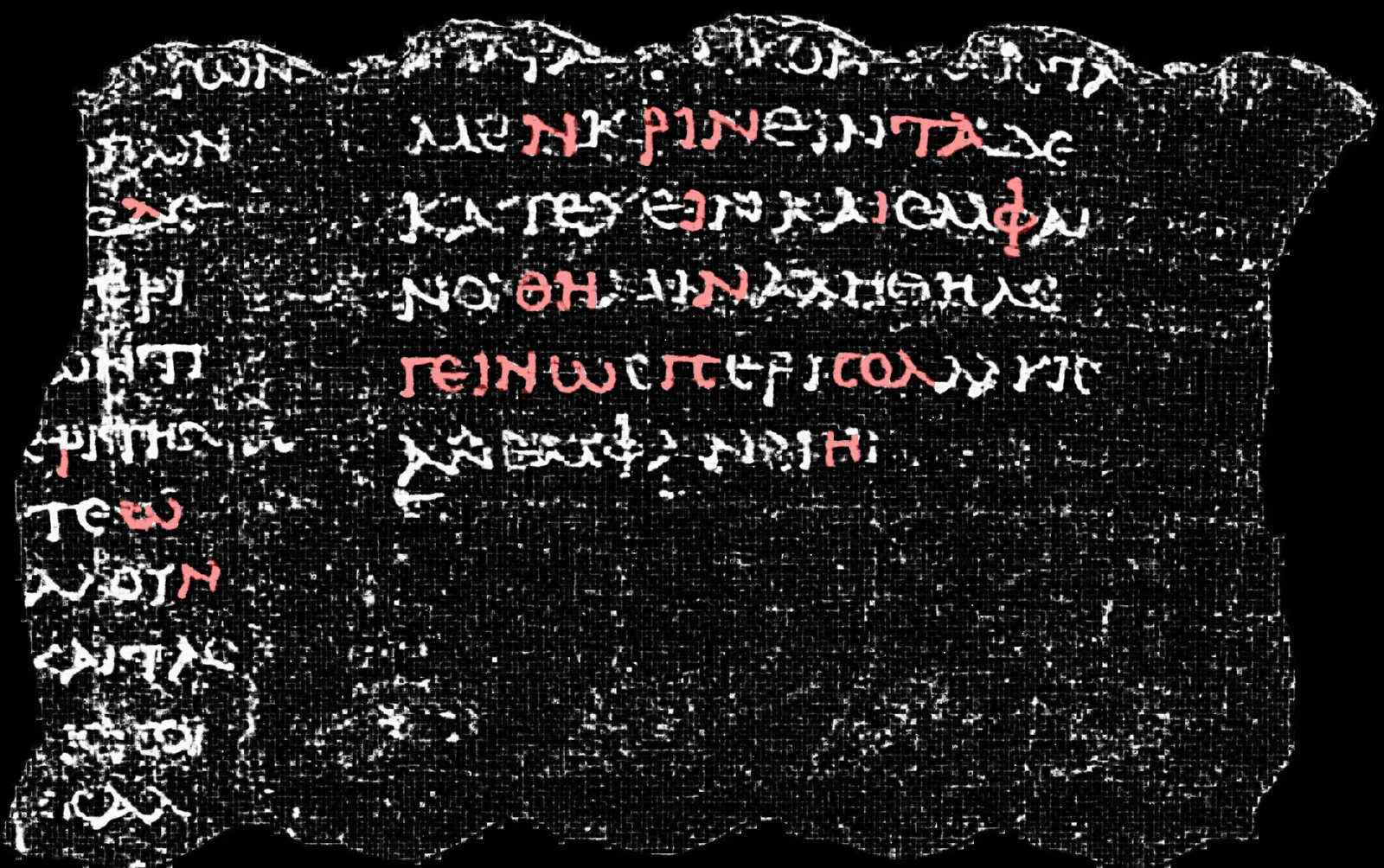
The three positional arguments are the segment's surface volume, the checkpoint (here the last one written by the 20,000-iteration run above), and the output path. (--overlap 0.5 --blend-mode hann spell out the defaults, 50% overlap with Hann blending, so the command stays reproducible.) The model slides across the whole segment in overlapping windows, blends the overlapping predictions, and writes a grayscale TIFF where each pixel's brightness (0–255) is the predicted probability of ink. Expect this to take on the order of an hour on a single GPU for a full segment. Open the result in any image viewer, and if all went well, you'll see letters, including outside the regions you had labels for.

tip

For a faster first look, pass --mask-path region.tif — a grayscale TIFF the size of the segment where nonzero pixels mark the region to predict — to limit inference to an area of interest.

Useful options:

• --gpus 0,1 — run on multiple GPUs.
• --tta-mirror — average predictions over mirrored versions of each patch (slower, slightly better).
• --layer-start / --layer-end — restrict which depth layers of the surface volume are used.
• --direction both — also write a depth-reversed prediction (as <output>_reverse.tif), useful when you aren't sure which side of the surface volume faces the ink.

Here is the result on the tutorial segment — the model's prediction in white, with the ink labels it was trained on overlaid in red:

The trained model's ink prediction for the tutorial segment. Red: the handful of letters it was trained on. Everything else it found on its own.

Native 3D: training and inference

Everything above is the 2.5D path: pre-rendered surface volume zarr in, 2D ink image out. The pipeline can also work natively in 3D, skipping the rendered surface volume entirely: for every training patch it uses the .tifxyz coordinates to find where the segment passes through the original scroll volume, samples a 3D crop there on the fly, and projects the 2D labels into the crop around the surface. The model then predicts ink directly in scroll space.

Two native 3D modes exist. full_3d trains on the raw crops; full_3d_single_wrap additionally feeds the model a second input channel marking which voxels belong to this segment's own wrap of papyrus, so the model isn't confused where neighboring wraps pass through the same crop — this is the mode to prefer.

Native 3D training

Create configs/ink_full3d.json. It is the same shape as the 2.5D config with a few changes: the mode, no z-projection (the prediction stays 3D), a full_3d block controlling the label projection, an on-disk cache for the streamed volume chunks, and a dataset entry that gains a volume_path pointing at the original scroll volume and trains at pyramid level 2 instead of full resolution:

{
  "out_dir": "runs/ink_full3d",
  "seed": 42,

  "mode": "full_3d_single_wrap",
  "model_type": "vesuvius_unet",
  "model_config": { "autoconfigure": true },
  "targets": { "ink": { "out_channels": 1, "activation": "none" } },

  "patch_size": [80, 128, 128],
  "patch_overlap": 0.5,
  "patch_min_labeled_coverage": 0.05,

  "full_3d": {
    "label_projection_half_thickness": 8,
    "background_projection_half_thickness": 8
  },

  "batch_size": 8,
  "num_iterations": 20000,
  "learning_rate": 0.01,
  "warmup_steps": 1000,
  "mixed_precision": "fp16",
  "dataloader_workers": 16,
  "prefetch_factor": 2,
  "pin_memory": true,

  "volume_cache_dir": "volume_cache",
  "volume_cache_max_gb": 120,

  "val_every": 1000,
  "save_every": 1000,

  "verify_finite_gradients_steps": 200,
  "max_amp_overflow_events": 4,

  "datasets": [
    {
      "segments_path": "/path/to/ink-dataset/phercparis4",
      "segments": ["w00_20231016151002"],
      "volume_path": "s3://vesuvius-challenge-open-data/PHercParis4/volumes/20260411134726-2.400um-0.2m-78keV-masked.zarr/",
      "volume_scale": "2"
    }
  ]
}

• volume_path is where the 3D crops come from. The public vesuvius-challenge-open-data S3 bucket is read anonymously — no AWS account needed. You can also download the volume locally (or just the chunks your segments touch, with vesuvius.ink_detection.preprocessing.download_required_zarr_chunks) and point volume_path at the local copy instead.
• volume_scale: "2" samples the crops from level 2 of the volume pyramid — 4× downsampled in each axis. That's enough for the tutorial; training at native resolution ("0") can bring further gains, at the cost of a much longer run. Distances in the config are always given in full-resolution voxels regardless of volume_scale — the pipeline converts them to the trained level internally.
• The full_3d block sets how far above and below the surface the 2D ink labels and supervision mask are projected into the crop, in full-resolution voxels (here ±8, so ±2 voxels at level 2).
• volume_cache_dir enables an on-disk LRU cache (capped at volume_cache_max_gb) for the chunks streamed from volume_path: each chunk is downloaded once and re-read from local disk afterwards, which makes both re-runs and inference (which shares the cache) much faster.
• There is no in_channels — the native 3D modes set it automatically before model construction. full_3d_single_wrap uses two input channels (the volume image and the reconstructed surface mask); plain full_3d uses one.

Training starts the same way:

uv run --extra models python -m vesuvius.ink_detection.training.train configs/ink_full3d.json

This run — 20,000 iterations at batch size 8 — takes about ten hours on an H100 with the tutorial segment.

tip

You don't have to wait ten hours to see results. Checkpoints land in the run folder every save_every iterations, so while training continues you can run the inference command below on an intermediate checkpoint, say ckpt_005000.pth, and watch the predictions improve from checkpoint to checkpoint.

Native 3D inference

Native 3D checkpoints use a different inference script, vesuvius.ink_detection.inference.infer_full3d_tifxyz, which samples patches the same way and writes a sparse 3D OME-Zarr prediction volume instead of a 2D image.

For inference the segment folder must contain a volume_source.txt — a single line with the path or URL of the original scroll volume:

echo "s3://vesuvius-challenge-open-data/PHercParis4/volumes/20260411134726-2.400um-0.2m-78keV-masked.zarr/" \
  > /path/to/ink-dataset/phercparis4/w00_20231016151002/volume_source.txt

Then, with your native-3D checkpoint, preview the work first: --plan-only validates the volume mapping and prints the occupied-chunk and patch counts without creating any output:

uv run --extra models python -m vesuvius.ink_detection.inference.infer_full3d_tifxyz \
  /path/to/ink-dataset/phercparis4/w00_20231016151002 \
  runs/ink_full3d/ckpt_020000.pth \
  predictions/w00_20231016151002_ink.ome.zarr \
  --resolution 2 \
  --overlap 0.5 \
  --batch-size 8 --num-workers 8 \
  --cache-dir volume_cache --cache-max-gb 120 \
  --plan-only

Even at level 2 a single segment plans tens of thousands of patches (the tutorial segment plans about 78,000; at full resolution it would be hundreds of thousands). When the printed patch count fits your compute budget, drop --plan-only and run the same command for real; the tutorial segment takes about two and a half hours on an H100.

• --resolution 2 must match the volume_scale the checkpoint was trained at.
• --num-workers 8 prepares patches in parallel worker processes, keeping the GPU supplied.
• --write-region occupied --chunk-halo 0 restricts the output to just the chunks that actually contain surface points, a useful optimization when you want a smaller, faster run than the default (which also writes a halo of neighboring chunks).
• For full_3d_single_wrap checkpoints, the script reconstructs the surface-mask input channel from the .tifxyz geometry automatically.

The result is an ink prediction in scroll coordinates rather than a flattened image:

Slicing through the prediction volume for the tutorial segment. The predicted ink follows the segment's wrap through the scroll.

To read it, render it through the segment geometry with VC3D's vc_render_tifxyz — the same tool that renders surface volumes from the scroll, just pointed at the prediction volume instead. You'll need a VC3D build on your PATH; see the VC3D tutorial's installation instructions.

vc_render_tifxyz \
  --volume predictions/w00_20231016151002_ink.ome.zarr \
  --group-idx 0 \
  --scale 1 \
  --scale-segmentation 0.25 \
  --segmentation /path/to/ink-dataset/phercparis4/w00_20231016151002 \
  --num-slices 16 \
  --slice-step 0.5 \
  --cache-gb 16 \
  --tif-output renders/w00_20231016151002_ink

This flattens the prediction into a stack of 16 slices spanning the surface, written as one TIFF per slice into the output folder. --scale-segmentation 0.25 maps the segment's full-resolution .tifxyz coordinates into the 4×-downsampled level-2 prediction volume. At that level, --slice-step 0.5 samples a focused band around the surface without accumulating as much papyrus texture as a wider step; use --slice-step 1 if you need to search farther along the normal. --scale 1 preserves the flat grid's output resolution. Finally, take a maximum over the slices to get a single readable image:

uv run --with numpy --with tifffile --with imagecodecs python -c "
import glob, numpy as np, tifffile
stack = np.stack([tifffile.imread(p) for p in sorted(glob.glob('renders/w00_20231016151002_ink/*.tif'))])
tifffile.imwrite('renders/w00_20231016151002_ink_max.tif', stack.max(axis=0))
"

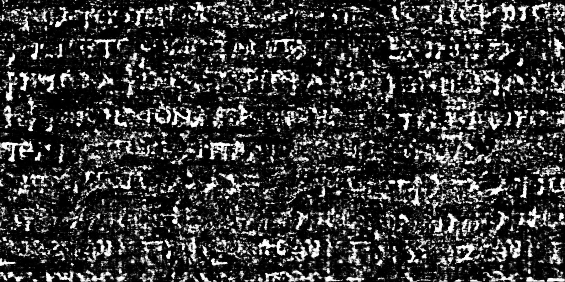
The model trained on a single segment, so the interesting test is a segment it has never seen. Here is the final checkpoint rendered this way on the central region of w05_4424, elsewhere in the scroll:

The 20,000-iteration checkpoint's prediction on a segment the model never trained on. Letters are starting to show, but this is still far from a good read.

The run above is a starting point. For better results, give the trainer more segments and train longer; the next section covers where to get them.

Scaling up: the full dataset

Everything above ran on one segment; scaling up is mostly a matter of downloading more. Sync a whole scroll (or several) into the same folder:

uvx --from huggingface_hub hf buckets sync hf://buckets/scrollprize/datasets/ink/phercparis4 ./ink-dataset/phercparis4

The training config doesn't change — segments_path already points at the folder, and the trainer picks up every segment in it on the next run. More segments means more diverse training data, which is the single most reliable way to improve the model.

For inference across many segments, use folder mode — it runs the checkpoint on every segment in the folder and writes each prediction into a preds/ directory inside that segment:

uv run --extra models python -m vesuvius.ink_detection.inference.infer \
  --folder /path/to/ink-dataset/phercparis4 \
  --checkpoint-path runs/ink_tutorial/ckpt_020000.pth \
  --batch-size 4

Improving the model: iterative labeling

A first model trained on a small dataset will reveal some letters clearly, others faintly, and miss some entirely. The way to make it better is the same loop that scaled ink detection to entire scrolls:

1. Run inference on your training segments (and new, unlabeled ones).
2. Inspect the predictions. Look for regions where letter strokes are clearly visible.
3. Extend the labels. In those regions, paint the visible strokes white in the ink label image, and extend the supervision mask to cover the region — both the strokes and the clean background around them, since the background pixels are the negative examples the model learns from.
4. Retrain on the enlarged labels, starting fresh or from your last checkpoint (add "checkpoint": "runs/ink_tutorial/ckpt_020000.pth" and "weights_only": true to the config).
5. Repeat.

Labels are ordinary image files, so you can edit them in any image editor that handles large images (e.g. GIMP or Photoshop). If you edit or create labels as TIFF/PNG files, convert them to the .zarr format the trainer expects with:

uv run --extra models python -m vesuvius.ink_detection.preprocessing.create_label_zarrs /path/to/ink-dataset/phercparis4

The figure below shows this loop in action on PHerc. 1667: with each iteration the labels (row a) grow from a handful of strokes to dense coverage, the model's predictions (row b) get cleaner, and the reading improves even on a held-out region that was never labeled (row c).

Pseudo-labeling process. Each column is an iteration. Model 0 is the starting point, not trained on PHerc. 1667. Row a: the training labels created from the previous iteration's inference. Row b: this iteration's prediction, with the labels used overlaid in magenta. Row c: the validation region, never used for creating labels. Source: the PHerc. 1667 paper.

Ink detection at 9 µm: pretrained cross-scroll models

Everything above trains a model on one scroll and runs it on segments of that same scroll. But the goal — and the open First Letters Prizes — is finding ink in scrolls nobody has read yet, where there are no labels to train on. For that, we share pretrained cross-scroll models: ink detectors trained on aligned labels from four scrolls (PHerc. 0139, PHerc. 1667, PHerc. Paris 4, and PHerc. 0814) at a common working resolution of roughly 9 µm isotropic.

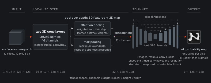
The models live at scrollprize/ink_9um on Hugging Face: a small local 3D stem feeding a 2D U-Net, trained twice with only the seed changed (hybrid_3d2d-seed42/ and hybrid_3d2d-seed43/), with seven checkpoints each along the training trajectory (step-010000.pth up to step-075000.pth). Different checkpoints behave a bit differently on different segments, so it's worth trying a few. Grab one to start:

uvx --from huggingface_hub hf download scrollprize/ink_9um \
  hybrid_3d2d-seed42/step-075000.pth --local-dir checkpoints/ink_9um

This section runs one of these models on a segment, starting from nothing but its .tifxyz surface geometry. That is the first-letters workflow: take a segment of an unread scroll, render it, run the shared models, and look.

Render your segment at 9 µm

The worked example is w035, a PHerc. 0139 segment from the models' own training set, so you know what a good result looks like before trying an unread scroll. Its .tifxyz is published on the open-data server (you can find it, along with every other public segment, in the Data Browser); for your own segment, use the .tifxyz you produced with VC3D instead:

aws s3 sync --no-sign-request \
  s3://vesuvius-challenge-open-data/PHerc0139/segments/20260317000000-w035_2026031718/mesh/20260317000000-on-20250728140407-9.362um.tifxyz/ \
  ink-dataset/pherc0139/w035/w035.tifxyz

Render the geometry against the scroll's native 9.362 µm volume with vc_render_tifxyz, the same tool that rendered the prediction volumes above. This time it streams the scroll volume from S3 and writes the surface volume as a Zarr. The 28-slice depth matches how the released segments on the data server are rendered; you can render deeper or shallower if you want to experiment:

vc_render_tifxyz \
  --volume volume-cache/20250728140407.zarr \
  --remote-url s3://vesuvius-challenge-open-data/PHerc0139/volumes/20250728140407-9.362um-1.2m-113keV-masked.zarr/ \
  --segmentation ink-dataset/pherc0139/w035/w035.tifxyz \
  --zarr-output ink-dataset/pherc0139/w035/w035_9um.zarr \
  --scale 1 --group-idx 0 --num-slices 28 \
  --cache-gb 16 \
  --voxel-size 9.362 --voxel-unit micrometer \
  --flip-normals

• --remote-url takes the S3 volume; --volume names a local directory where fetched chunks are cached, so only the parts of the scroll your segment touches ever get downloaded. --voxel-size and --voxel-unit record the physical metadata the remote volume can't provide.
• --flip-normals reproduces the depth orientation of the published renders and the training labels; for your own segment the orientation is unknown, which is what --direction both at inference time is for.

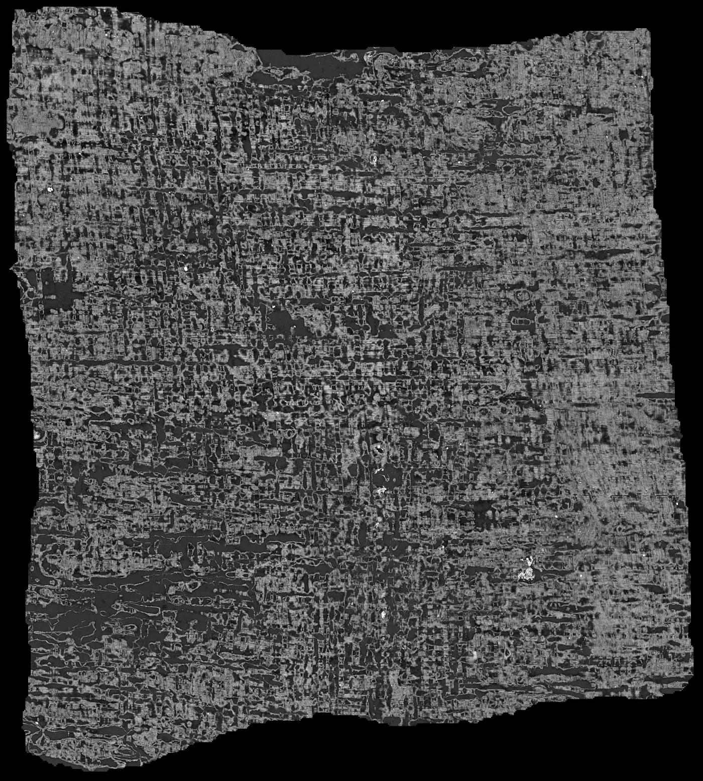
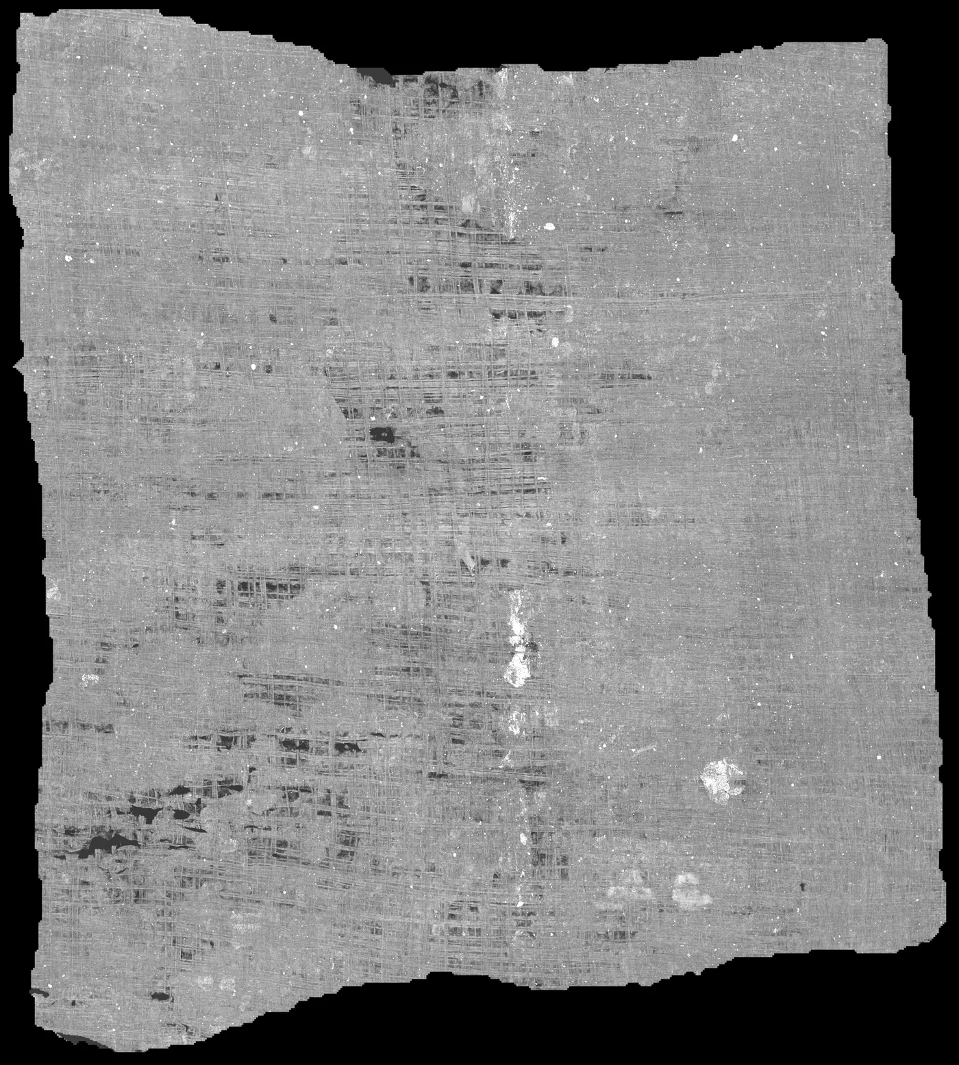
For w035 this takes about five minutes and writes a ~900 MB Zarr:

(a) Middle slice

(b) Max projection over depth

The rendered w035 surface volume: 28 slices of 5820×5240 at 9.362 µm. No ink is visible to the eye; that's the model's job.

tip

If you are already in VC3D, you don't need the command line for this: right-clicking a segment and choosing Render runs the same vc_render_tifxyz under the hood, with the same parameters in a dialog.

(For w035 the rendered surface volume is also already published, under the segment's surface-volumes/ folder on the data server, so you can skip the render and try the model immediately.)

Run the models

The rendered surface volume goes through the same flat inference command as before; only the input and the checkpoint change:

uv run --extra models python -m vesuvius.ink_detection.inference.infer \
  ink-dataset/pherc0139/w035/w035_9um.zarr \
  checkpoints/ink_9um/hybrid_3d2d-seed42/step-075000.pth \
  predictions/w035_9um.tif \
  --overlap 0.5 --blend-mode hann \
  --batch-size 32

The --batch-size 32 assumes a large GPU; drop it to 4 or 1 if you run out of memory.

Checkpoints embed their training config, so inference rebuilds the model and its normalization automatically. Two things to know when reading the output:

• The models are sensitive to depth offsets. If a checkpoint doesn't respond well on your data, the surface may sit at a slightly different depth than the model expects. Try shifting the window with --layer-start / --layer-end, or average the predictions over a few nearby windows as a simple ensemble. Training jitters the depth window, so the models tolerate small offsets; larger ones can still throw them off.
• The background doesn't sit at zero. With label smoothing 0.5, the training targets are 0.25 for background and 0.75 for ink, so predictions tend to occupy a compressed range. If a prediction looks washed out, you may want to rescale it for display (for example (p − 0.25) / 0.5, clipped to [0, 1]).

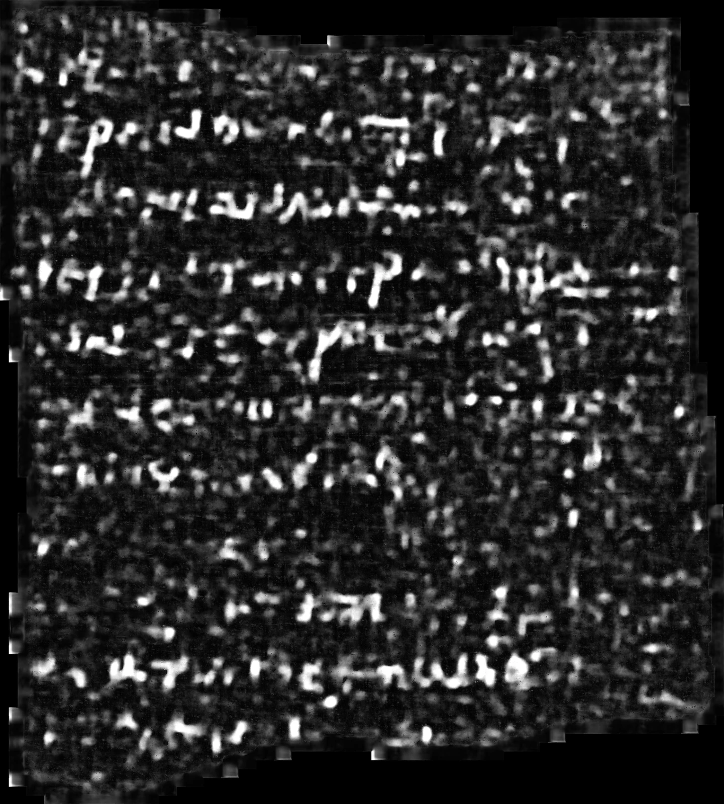
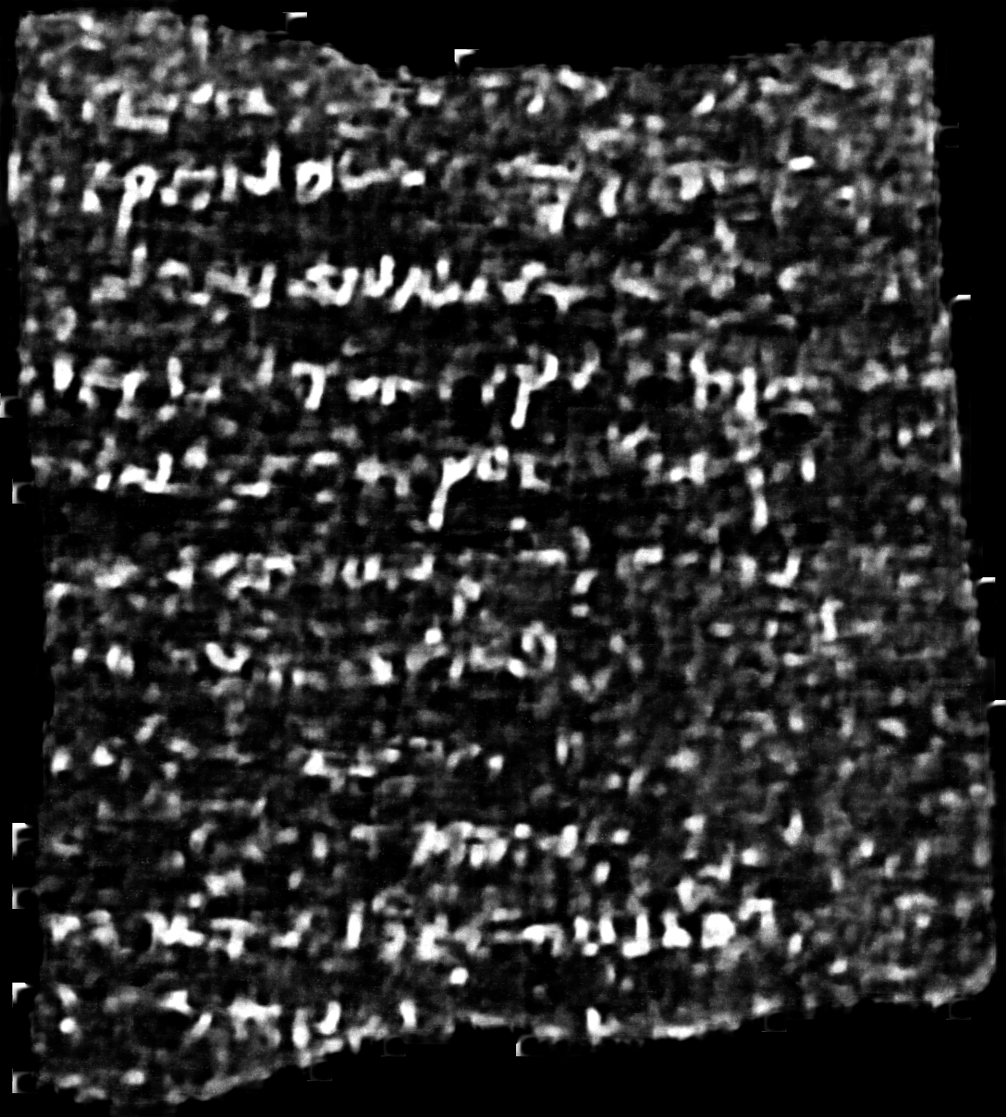
Run both seeds and a few different steps; and when you don't know which way the surface faces, run both directions too (--direction both). Here is how the two seeds compare on the w035 render from above:

seed 42

seed 43

The two seeds on the w035 surface volume, both at checkpoint step-020000, rescaled for display. Drag to compare.

Train the 9 µm recipe yourself

There is plenty of room to improve on these models: better augmentation, longer training, other architectures, ensembling, and more data are all open directions. The full training setup is public. The labels live in the ink_9um dataset:

uvx --from huggingface_hub hf buckets sync hf://buckets/scrollprize/datasets/ink_9um ./ink_9um

It contains labels only: 24 segments annotated on pooled 2.4 µm renders (labels/aligned-scrollprizeorg-21slices/) and 5 on native 9.362 µm renders (labels/native9-scrollprizeorg-21slices/), in exactly the segment-folder layout the trainer consumes. The surface volumes come from the open-data server; the dataset README's per-segment tables say which public volume each segment annotates.

The full recipe lives in a single config file. Copy src/vesuvius/ink_detection/configs/aligned21_hybrid_3d2d.json from the repo into your configs/ folder. It defines the hybrid 3D→2D model, a jittered 17-of-21 depth window, robust normalization, and batches drawn with fixed per-scroll quotas (29/22/11/2 of 64), and its datasets block already lists all 29 training representations: 24 aligned and 5 native, covering 25 physical segments. What it expects from you is each segment's surface volume, at <segment>/surface-volume.zarr next to its labels: the native 9.362 µm renders are used as they come from the server, and the 2.4 µm ones are first pooled to ~9.6 µm with python -m vesuvius.ink_detection.preprocessing.prepare_9um_isotropic_input <in.zarr> <out.zarr>. Point the /path/to/ink_9um placeholder at your synced folder, set out_dir, and train:

uv run --extra models python -m vesuvius.ink_detection.training.train configs/aligned21_hybrid_3d2d.json

The full 78,125-iteration run takes about five hours on one H100. To add your own data, label your segments with the same iterative loop from the previous section, place them beside the downloaded ones, and add them to a datasets entry. If your scroll mix differs from the released one, adjust (or remove) the fixed_scroll_prior quotas: the sampler enforces the per-batch scroll counts and fails fast on a scroll it has no data for.

What's next

With segmentation and ink detection you now have the complete pipeline: from a 3D X-ray scan of an intact scroll to readable text. This exact loop — better segments, more careful labels, retrained models — is what produced the complete reading of PHerc. 1667, and there are hundreds of scrolls to go.

Join the Discord to see what the community is working on, check the open prizes, and help us read the rest of the library.