Tutorial: Representation
This page has been archived and is no longer maintained. It describes an earlier generation of the Vesuvius Challenge pipeline — tools, data layouts, and results referenced here may have been superseded. See Open Problems for the current state of the pipeline and Prizes for what is open today.
The micro-CT scan converts the scroll into a volumetric grid of density measurements, providing a mathematical description with integer coordinates and average material densities in small adjacent cubes known as voxels.
While the raw scan volume represents the maximum amount of information available, this dataset is huge and the papyrus surface is difficult to locate throughout the scroll. Mathematical calculations and machine learning can be used to manipulate the digital dataset into different representations that are easier to interpret both visually and computationally.
Besides the raw scan volume, three types of representations have been explored:
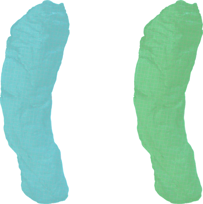
- Machine Learning Segmentation
- Traditional voxel processing
- Point Clouds
Input: 3D scan volume (voxels in .tif “image stack”)
Output: binary 3D volume (voxels in .tif “image stack”)
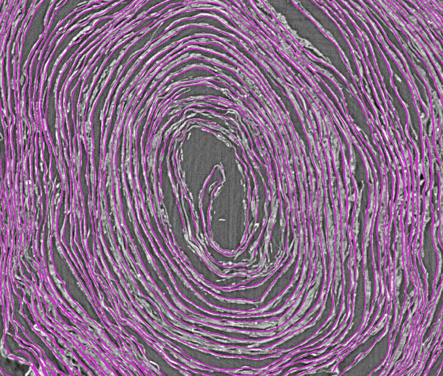
Machine learning segmentation involves separating the part of the papyrus we wish to work with from the rest of the scan. We have trained models on a number of different papyrus features, but our current methods focus on two structures that exist within the scroll: The recto (inside) or verso (outside) surfaces, and the fibers which make up the papyrus sheet itself.
In the image below, the purple lines mark the recto surface, giving us a much more tractable representation to work with on downstream tasks than the scan itself.
Input: 3D scan volume (voxels in .tif “image stack”)
Output: new 3D volume (voxels in .tif “image stack”)
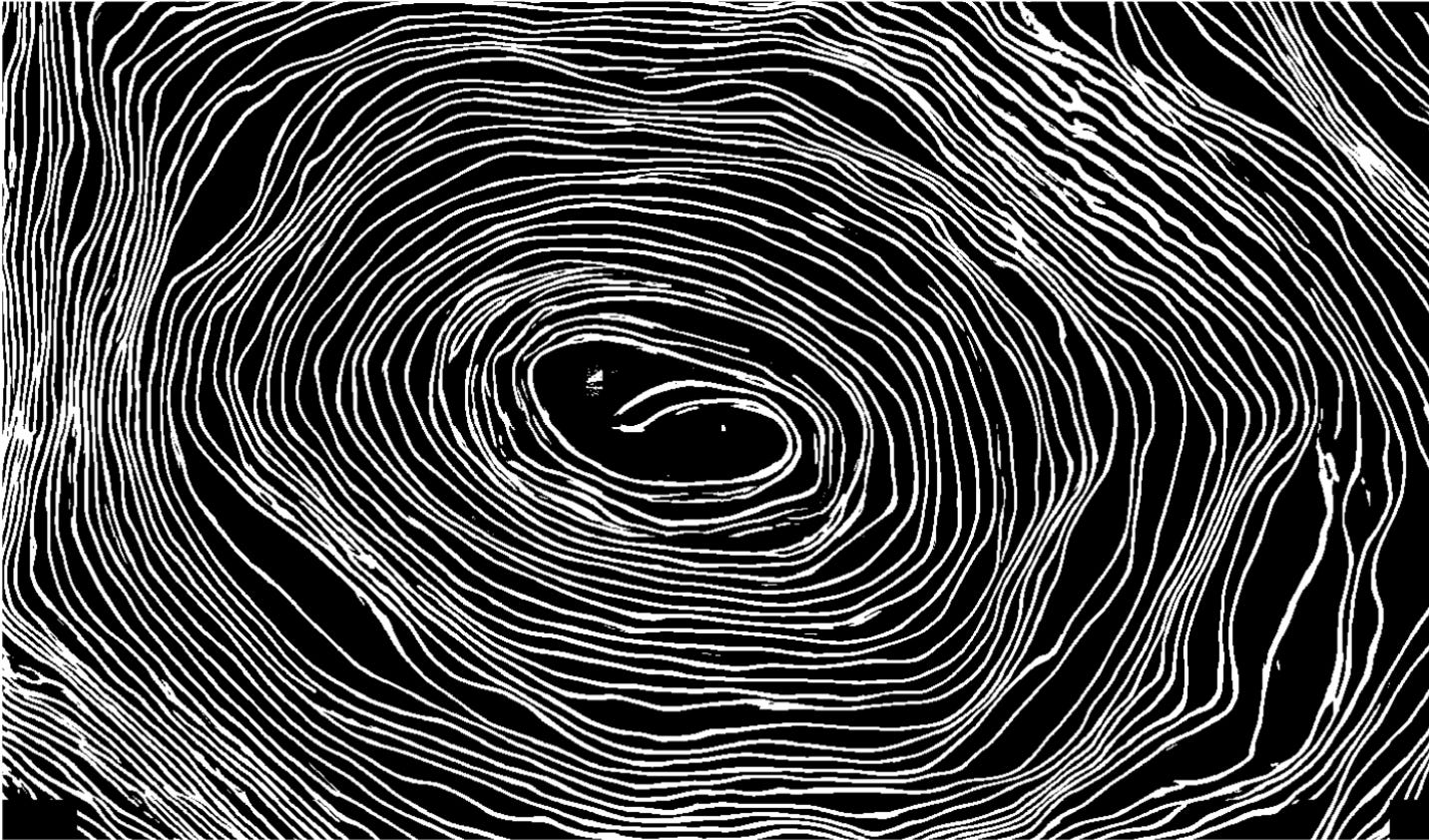
Traditional image processing techniques have mostly been intended to aid manual segmentation, either to make the papyrus easier to interpret or to help segmentation algorithms follow the surface better. Popular techniques include thresholding, noise reduction, various colourization schemes, edge detection, and skeletonization.
Most of these techniques have not been successful at improving segmentation.
Input: 3D scan volume (voxels in .tif “image stack”)
Output: point cloud (.ply or .obj)
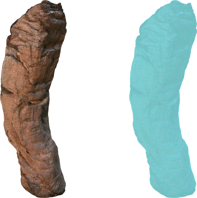
The goal of point clouds is to extract a limited but useful subset of information from the raw scan volume. In the point cloud representation, calculations select voxels that describe the surface of a sheet.
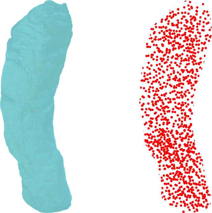
The fixed grid and density values are discarded, using traditional edge/surface detection to generate infinitesimal points characterized by 3D real coordinates. If needed, the discarded information can be reattached to the points to revert to the voxel representation.
Semantic Segmentation of Scroll Structures
This guide will focus on utilizing machine learning to create semantic segmentations of recto surfaces, but the same methods apply to any of our other datasets, such as fibers -- simply swap out the training images and their associated labels. It is written using Ubuntu 22.04, but the guide should translate to most any version of Linux. Windows users are advised to use WSL2 and place their data within the Linux filesystem.
For this tutorial, we'll be using a library/framework known as nnUNetv2
nnUNet is a well regarded and highly performant machine learning library with a focus on volumetric data within the medical domain, which has many parallels to our imaging modalities (namely xray tomography), and provides us with a fantastic baseline and starting point for experimentation.
This is a simplified guide, it is highly recommended to visit the repository and read further after following this!
Installing nnUNet and its Dependencies
Requirements
- Working CUDA installation -- Installation instructions
- Nvidia GPU with 10GB VRAM
- 32GB CPU RAM (although you may be able to get by with a bit less)
If you do not already have a virtual environment manager, install miniconda:
wget https://repo.anaconda.com/miniconda/Miniconda3-latest-Linux-x86_64.sh

bash Miniconda3-latest-Linux-x86_64.sh -b -p $HOME/miniconda3

source $HOME/miniconda3/bin/activate
Create a virtual environment for nnUNet:
conda create -n nnunet python=3.10
conda activate nnunet
Install Pip within the Conda Environment (this is done because PyTorch no longer creates Conda packages)
conda install pip
Install PyTorch
pip install torch torchvision
Install nnUNetv2. If you wish to extend nnUNet, you can install in editable mode by following these instructions
pip install nnunetv2
Data Preparation and Preprocessing
Download and extract the test dataset. Choose a folder you'd like to store your nnUNet data in, and structure the folders like so, placing the dataset where indicated in the tree:
.
└── nnUNet_data/
    ├── nnUNet_raw/
    │   └── Dataset060_s1_s4_s5_patches_frangiedt_test/
    │       ├── imagesTr
    │       ├── labelsTr
    │       └── dataset.json
    ├── nnUNet_preprocessed
    └── nnUNet_results
You may notice by now that the images contain a suffix of _0000 while the labels do not. This suffix maps the images to a normalization scheme defined in dataset.json, for more information if desired, visit this page.
nnUNet requires some information about where you have stored this dataset, which it accesses from environment variables. Set them for the current session with the following commands. You can make them permanent if you'd like by adding the same lines to your ~/.bashrc file.
export nnUNet_raw="/path/to/nnUNet_data/nnUNet_raw/"
export nnUNet_preprocessed="/path/to/nnUNet_data/nnUNet_preprocessed/"
export nnUNet_results="/path/to/nnUNet_data/nnUNet_results/"
Now we can begin the preprocessing stage. nnUNet will gather some information about your dataset, verify there is nothing wrong with it, and extract it into uncompressed numpy arrays.
nnUNetv2_plan_and_preprocess -d 060 -pl nnUNetPlannerResEncM
This can take a few minutes, and will print some information as it goes. It should finish without errors.
Training
With our data preprocessed we can finally begin training. The command here will begin a training run using dataset 060 (the identifier for our test dataset), using the 3d_fullres configuration, and fold 0.
nnUNet automatically creates 5 training folds for cross-validation on your dataset, and these splits can be modified in the splits_final.json which is generated after initiating training. You can run without any cross-validation by specifying all instead of a fold number.
nnUNetv2_train 060 3d_fullres 0 -p nnUNetResEncUNetMPlans
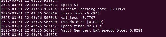
nnUNet will extract the dataset, and begin training at epoch 0. While training runs it will print the progress in the terminal. The EMA pseudo dice is computed on a random validation batch, and shouldn't be taken as gospel, but can provide a relative idea of how well the training is going, provided you have not used the all fold.
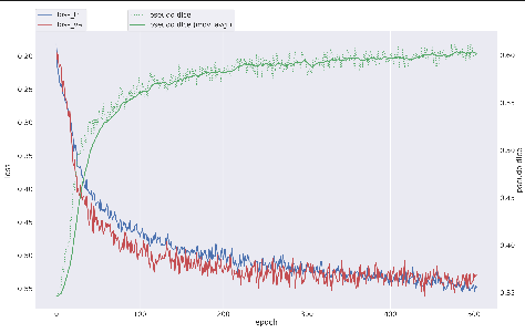
nnUNet will also store a graph that can be used to assess the current training run located in /path/to/nnUNet_data/nnUNet_results/Dataset060_s1_s4_s5_patches_frangiedt_test/nnUNetTrainer__nnUNetResEncUNetMPlans__3d_fullres/fold_0/progress.png
This contains information about current learning rate and epoch time, but of particular interest is the top graph containing information about current psuedo dice and training and validation loss. Ideally, your bar should look like this -- where both training and validation loss are continuing to drop along similar paths.
Towards the end, you can see my training loss continues to drop while my validation loss levels out, this tells us that the model is no longer improving on the validation data, and is likely beginning to overfit to the training data. This is not necessarily bad, but you would not want these lines to diverge too greatly. You can end training at any time by pressing ctrl+c in the terminal window, or allow training to continue for the default max_epochs, which for nnUNet is 1,000.
Inference
To run inference with your newly trained model, you first need to ensure that the file names contain the same suffix as the ones you trained with. In our case, this is _0000. This example will run inference on all of P.Herc. 1667 to show the process of reconstructing the inference back to the original volume, you can simply download a single grid and run inference on only one if you only wish to see what the inference output looks like!
Download the Scroll 4 grids. These are 600x600x600 volumes, with the same naming convention as the original scroll grids, but with 50 voxels of overlap in all directions so that when we reconstruct it we can do so in a way that mitigates edge artifacts. Inference on this entire volume takes around 13 hours on two RTX 3090s.
If you stopped your training early, you'll need to go into the results folder in your nnUNet_results path, and change one of the checkpoints to checkpoint_final.pth
Place the data in any folder, and run the command
nnUNetv2_predict -d 060 -f 0 -c 3d_fullres -i /path/to/input/grids -o /path/to/output/grids -p nnUNetResEncUNetMPlans
for multi-gpu setups, you can run inference like so, repeating for as many gpus as you have available
CUDA_VISIBLE_DEVICES=0 nnUNetv2_predict d 060 -f 0 -c 3d_fullres -i /path/to/input/folder -o /path/to/output/folder -p nnUNetResEncUNetMPlans -num_parts 2 -part_id 0  &

CUDA_VISIBLE_DEVICES=1 nnUNetv2_predict d 060 -f 0 -c 3d_fullres -i /path/to/input/folder -o /path/to/output/folder -p nnUNetResEncUNetMPlans -num_parts 2 -part_id 1
To export the probabilities, append --save_probabilities to the end of the inference commands. This will save an npz and a pkl file, which you can turn into uint8 tifs with this script
Once inference has completed, download this script, and in the main block, change map=False to map=True, and change Scroll='1' to Scroll='4'. This will modify the pixel values of your inference (which are simply 0 for background and 1 for foreground) to 0 and 255, and map your grids to the proper volume shape. You can modify max_workers and chunk_size if desired.
python grids_to_zarr.py
This script will add your blocks to a zarr array of the proper shape, and trim the 50 voxel overlaps we added previously. The result of this is a single resolution zarr. It is recommended to create a multi-resolution ome-zarr , by using this script, written by Discord member @khartes_chuck.
python zarr_to_ome.py /path/to/single_resolution.zarr /path/to/multi_resolution_ome.zarr --algorithm max
The final result is the predicted recto surface for the entirety of Scroll 4 that should be much easier to work with than the original scan data in downstream tasks. Volumes like this one are the inputs for methods used in our next guide on segmentation.