Tutorial: Spiral Fitting

Last updated: July 9, 2026

Content feeling overwhelming? Catch up by asking Philodemus.

Most of our segmentation tools work bottom-up. GrowPatch, lasagna, and manual segmentation in VC3D all produce patches — pieces of papyrus surface that you grow bigger and bigger until they hit a tricky region and stall. Other tools trace individual fibers. Either way you end up with a big pile of small pieces: segments, fibers, point annotations. What we really want is the whole scroll — one surface covering every winding of the original papyrus sheet, from the center to the outer shell. However, gluing the pieces together directly is hard, especially where there are gaps between them. ¹

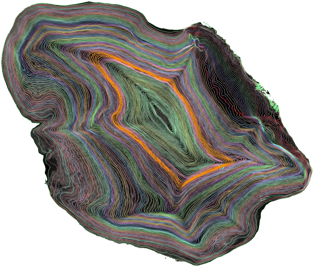
That is what the spiral fit does. It takes the whole pile of partial evidence — surface patches, traced lines, winding annotations, volumetric predictions — and fits a single, globally coherent surface for the entire scroll that agrees with as much of that evidence as possible. Where the evidence is dense, the fitted surface follows it closely; where there are gaps, the spiral bridges them smoothly instead of stopping or leaving a gap.

The result of fitting a spiral to PHerc. Paris 4 (Scroll 1): the 130 fitted windings, overlaid on a horizontal slice through the scan.

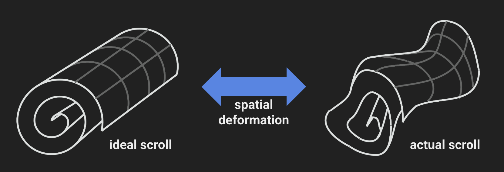
The core idea: we know the scroll was originally one long rectangular sheet, rolled up into a neat spiral. The eruption of Vesuvius deformed that spiral into the crushed shape we see in the CT scan. Instead of reconstructing the surface piece by piece, we search for the combination of ideal scroll shape and smooth deformation that best explains everything we observe. Once we have those, virtual unrolling comes almost for free: any point in the scan can be mapped back onto the original flat sheet.

The last section of this tutorial goes into how it works internally; first, the practical part — what goes in, what comes out, and how to run it.

What goes in

The spiral is flexible about its inputs: it consumes many kinds of evidence, in almost any combination, and each kind can be created manually or automatically.

• Surface patches — small pieces of scroll surface, stored as tifxyz meshes (the grid-of-3D-points format used by VC3D). These can come from GrowPatch, lasagna (direct growth, or growth around fibers), neural Copy In/Out, or any other segmentation method. Patches are split into two groups, verified and unverified: the fit places strong weight on the human-checked verified patches, and treats the unverified ones as weaker hints. The verified patches are also used to calculate evaluation metrics.
• Strips and lines of points that follow the surface of a single sheet — either point collections drawn in VC3D, or fibers traced in VC3D.
• Relative winding annotations — sets of points lying on different windings, annotated with how many windings apart they are (e.g. "these two points are exactly one wrap apart"). Represented as VC3D point collections with relative-winding annotations.
• Absolute winding annotations — points annotated with the absolute winding number they lie on (e.g. "this patch is on winding 20"). Also VC3D point collections.
• Coarser volumetric guidance derived from machine-learning predictions: predicted surface normals (from lasagna, stored as zarr volumes), predicted gradient magnitude (which captures the local radial density of windings), and skeletonised surface-prediction tracks (created with extract_surface_tracks.py).
• Scroll-level structure: the umbilicus (the scroll's central axis, as a function of z — required), and optionally a mesh of the scroll's outermost surface, which pins down where the spiral must end.

Multi-winding annotations.

Same-winding fiber annotation.

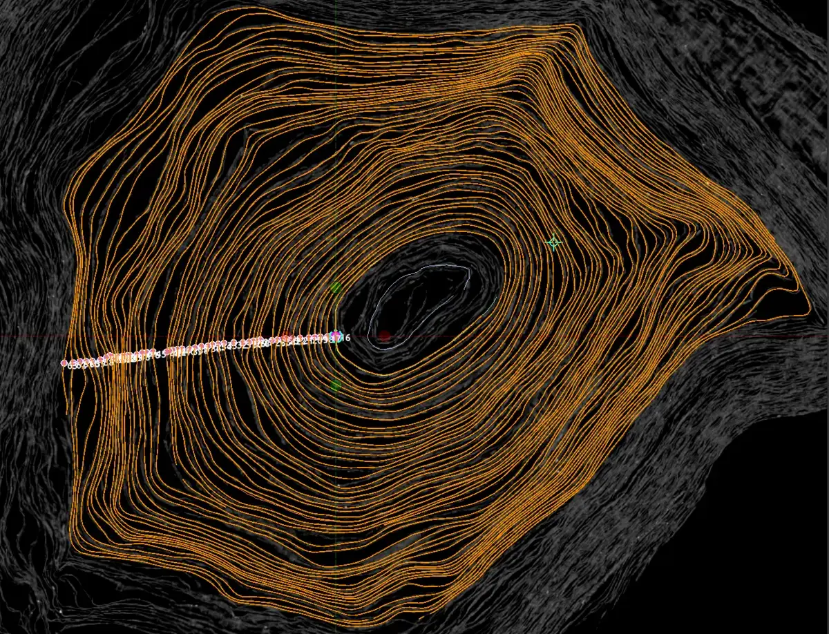
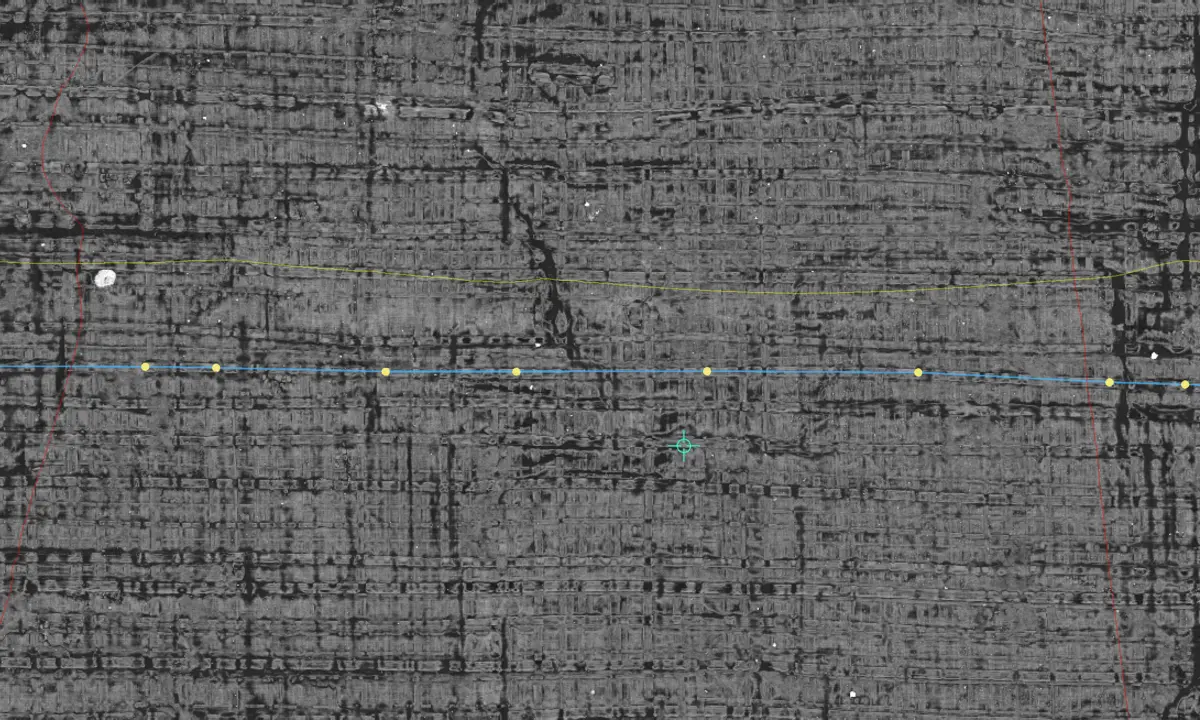
None of these individually needs to cover the scroll. Sparse, scattered evidence — a patch in one region, a fiber in another, a few relative-winding annotations in an ambiguous area — is combined by the fit into one consistent global solution, and annotations placed where the scroll is most damaged contribute the most.

What comes out

The output is one tifxyz mesh per winding of the scroll — a full set of surfaces that conform to the input constraints, covering the whole fitted region including places no patch ever reached. Two variants are written for each winding: wNNN, the pure fitted spiral surface, and wNNN_spliced, where the geometry of verified patches is spliced into the fitted surface wherever the fit and the patch agree — more locally accurate wherever trusted geometry exists.

Since these are ordinary tifxyz meshes, everything downstream works as usual: you can load them in VC3D, flatten them, and render surface volumes for ink detection. The repo also includes a tool (render_ink.py) that concatenates the windings into fixed-width chunks, flattens them, and renders ink predictions as a series of horizontal strips — more on that below.

Alongside the meshes, a fit writes a model checkpoint, overlay images showing the fitted windings drawn over scan slices, and satisfaction metrics — per-input-type statistics of how much of the evidence the final surface actually honors.

How to run it

The code lives in the villa repository under volume-cartographer/scripts/spiral; the main entry point is fit_spiral.py. You'll need Python ≥ 3.14 and an NVIDIA GPU.

git clone https://github.com/ScrollPrize/villa.git
cd villa/volume-cartographer
uv pip install torch torchvision   # pick the build matching your CUDA version
uv pip install -e scripts/spiral   # the spiral scripts' Python dependencies
uv pip install -e .                # volume-cartographer python bindings

The spiral scripts declare their dependencies in their own pyproject.toml — only torch is left for you to install, so you can pick the right build for your CUDA version. The last line builds the volume-cartographer Python bindings, which the fit uses to link point annotations to patches; it compiles C++, so you'll need cmake and VC's build dependencies (see the segmentation tutorial if it fails).

Get the dataset

Ready-made inputs for PHerc. Paris 4 (Scroll 1) are published in the spiral-input dataset, which lives in the scrollprize/datasets storage bucket on Hugging Face (~50 GB):

uvx --from huggingface_hub hf buckets sync \
  hf://buckets/scrollprize/datasets/spiral/PHercParis4 \
  ./spiral-dataset/PHercParis4

hf buckets sync works like rsync: re-running it resumes interrupted downloads. The dataset contains verified and unverified patches, tracks, fibers, the outer shell, winding annotation JSONs, the umbilicus, and the volume inputs — see the dataset README for the exact layout.

Configure

Configuration is straightforward: the input paths and fitting region are plain variables at the top of fit_spiral.py. Edit them to point at your download:

• dataset_path — the root of the dataset; the per-input paths below it (verified_patches_path, unverified_patches_path, pcl_json_paths, fibers_path, shell_path, tracks_dbm_path, the normals/grad-mag zarr paths, …) default to locations inside it. Set any of them to None to fit without that input.
• z_begin, z_end — the slice range (in full-resolution voxels) to fit. Consider starting with a small range: the whole written region of Scroll 1 is roughly z 4,000–17,000, and fitting all of it needs a lot of GPU memory (around 60 GB). A ~1,000-slice range is a good first run on a smaller GPU. Per-step sample counts are scaled automatically to the size of the z-range, so hyperparameters don't need retuning when you change it.

Everything else — loss weights, resolutions, step counts — lives in the default_config dict just below, with one entry per knob. You can override any of them without editing the file via a JSON environment variable, and a few other environment variables control the run:

Variable	Effect
FIT_SPIRAL_CONFIG_OVERRIDES	JSON dict of default_config overrides, e.g. '{"num_training_steps": 10000}'
FIT_SPIRAL_OUT_DIR	Output directory (default ./out)
FIT_SPIRAL_CACHE_DIR	Cache for preprocessed inputs (default ../cache) — speeds up subsequent runs a lot
FIT_SPIRAL_RUN_TAG	Tag appended to the output folder and mesh names
FIT_SPIRAL_RESUME_PATH / FIT_SPIRAL_RESUME_STEP	Resume from a checkpoint
WANDB_MODE	Set to online to log losses and visualizations to Weights & Biases (default disabled)

Fit

python fit_spiral.py

That's it — the script loads the inputs (caching the expensive preprocessing), then runs 30,000 optimization steps, printing the loss breakdown every 200 steps. Multi-GPU is supported via torchrun --nproc-per-node=N fit_spiral.py, which splits each step's work across GPUs.

When it finishes, you get a self-contained run folder:

out/2026-07-08_s1_slice-10500-11500_27399-patch_<run-name>/
├── checkpoint_fitted.ckpt        # fitted model (resumable)
├── spiral_on_*_fitted.png        # fitted windings overlaid on inputs
├── satisfied_fitted.json         # how much of each input the fit honors
└── meshes/mesh/
    ├── w010/                     # one tifxyz mesh per winding...
    ├── w010_spliced/             # ...plus the patch-spliced variant
    ├── w011/
    └── ...

Rendering ink

To get from per-winding meshes to readable images, use render_ink.py. It groups the _spliced winding meshes into winding-range chunks, concatenates each chunk into a single mesh (written to a concat/ folder — useful for loading the geometry behind each strip as one mesh), SLIM-flattens it, renders it through an ink-prediction volume with vc_render_tifxyz, and composites the result into one JPEG strip per chunk:

python render_ink.py /path/to/run/meshes/mesh --volume /path/to/ink_prediction.zarr

You'll need a VC3D build on your PATH for the rendering and flattening binaries (vc_render_tifxyz, flatboi, …), and an ink-prediction zarr for the scroll. The output ink/ folder fills with strips named by winding range (e.g. w010-027.jpg).

Ink metrics

The script get_ink_metrics.py computes some metrics based on the amount of letter-like ink signal detected in the ink renders. By default it uses the model scrollprize/ink-coverage-32um from HuggingFace; this is a 2D nnUNet operating on small patches, trained to do binary segmentation of clearly-identifiable ink. The script measures the total area of ink detected, as well as evaluating whether columns are coherent and have approximately the expected width, and lines are locally coherent (based on sliding windows) and have approximately the expected pitch.

warning

The ink-coverage model was only trained on PHerc. Paris 4, so it may not give accurate results for other scrolls with significantly different writing styles.

How it works

Up to this point we treated the fit as a black box; here is what is actually inside it. (There are more math details in the paper Virtually Unrolling the Herculaneum Papyri by Diffeomorphic Spiral Fitting, though for a slightly older version of the algorithm.)

An ideal scroll...

Originally, a scroll was one nearly rectangular sheet of papyrus, rolled up (often around a central rod). In cross-section that is a spiral — specifically, we model it as a perfect archimedean spiral, extruded into the plane. Treating it as arbitrarily large, the ideal scroll has just one free parameter: the tightness of its windings, $\omega$. A point on the ideal sheet is addressed by two curvilinear coordinates — the angle $\theta$ along the spiral and the height $z$ along the axis — and sits at radius

$$r(\theta) = \tfrac{\omega}{2\pi}\,\theta,$$

so each full turn moves the sheet outward by one sheet-to-sheet spacing $\omega$. Plug in any $(\theta, z)$ and you get a 3D point on the ideal sheet.

...horribly deformed

The eruption turned that neat spiral into the crumpled shape in the scan. We model the damage as a diffeomorphic transformation: a smooth, differentiable, invertible map of 3D space. That choice buys us exactly the guarantees we need:

• It cannot tear the sheet, make it pass through itself, or squish it to a point — it preserves topology. If it starts as a spiral, after deformation it is still a spiral, just a messed-up one.
• It is invertible: a point on the ideal scroll maps to a point in the scan, and — just as importantly — any point in the scan maps back to a point on the ideal (i.e. flattened) scroll. That inverse map is the virtual unrolling.

The deformation is composed of three parts applied in sequence: a coarse global scale and shear, the integral of a stationary velocity field (the most important one), and a local scaling of the gap between windings, defined everywhere on the sheet (this lets windings locally squeeze together or spread apart without disturbing anything else). Each part is smooth and invertible, so the composition is too.

The middle term deserves a closer look. Imagine a little 3D arrow attached to every point in space — a velocity field $u$. Every point of the ideal spiral flows along these arrows, like dust in a (smooth, steady) wind. Mathematically, the trajectory $\phi_t(x)$ of a point $x$ is defined by the ODE

$$\frac{\mathrm{d}\phi_t(x)}{\mathrm{d}t} = u\big(\phi_t(x)\big), \qquad \phi_0(x) = x,$$

and the transformation is where the flow ends up after one unit of time: $T_{\text{flow}}(x) = \phi_1(x)$. Don't worry too much about the equation — the intuition is what matters: every point rides smoothly along the flow, so the whole spiral deforms smoothly into a new shape, and running the flow backwards gives the exact inverse. This is the same machinery used in diffeomorphic medical image registration; in the code, the ODE is integrated with a few Runge–Kutta steps (flow_fields.py, transforms.py).

An idealized rolled scroll (left) is related to the deformed scroll observed in the scan (right) by a smooth spatial deformation — the transformation the spiral fit estimates.

Fitting as an inverse problem

Fitting is then an inverse problem: find the winding tightness $\omega$ and the deformation parameters (the velocity field, plus the scaling terms) such that the deformed spiral explains what we see in the scan. We don't fit to the raw CT intensities directly. Instead, every input from What goes in becomes a differentiable loss term saying what the deformed spiral should look like:

• points from a same-sheet strip should all land on some winding surface (and the same one);
• two points annotated as $k$ windings apart should land exactly $k$ windings apart;
• a verified patch should coincide with a single winding across its whole extent — with unverified patches pulled in more gently;
• tracks, normals, and gradient-magnitude volumes nudge the surface orientation and winding density;
• the innermost winding should wrap the umbilicus, and the outermost should follow the outer shell;
• and regularization terms keep the sheet parameterization from distorting.

All parameters are optimized jointly, with plain Adam, minimizing the weighted sum of these losses (the weights are the loss_weight_* entries in default_config). In effect, we tell the machine "here are all the constraints humans and models have gathered — find the deformation that squishes the ideal spiral so that they are all met", and gradient descent does the rest.

At the end, we sample each winding of the fitted ideal spiral on a regular $(\theta, z)$ grid, push the samples through the fitted deformation into scan coordinates, and write each winding out as a tifxyz mesh — the outputs described above.

One caveat when reading the paper: it describes a fully automatic setup that fits only raw surface-prediction tracks and fields derived from them. The current code fits the much richer curated evidence described in this tutorial — verified patches, fibers, and winding annotations — which is what makes it accurate enough to target whole-scroll segmentation. The underlying model and optimization are still very similar.

Footnotes

1. The surface tracer is an earlier attempt at this problem: it stitches overlapping patches into large segments automatically. But it requires the patches to physically overlap or touch, and it becomes unreliable at whole-scroll scale. ↩