Open Problems: Why Reading Every Herculaneum Scroll Is Still a Challenge
Last updated: July 10, 2026
In 2026, PHerc. 1667 was virtually unwrapped and read without physically opening the scroll (see References).
We are no longer asking whether a sealed Herculaneum scroll can be read. It can. The harder question is how to make the same process work automatically, reliably, and at scale for every scroll.
🙋 How you can help
This post doubles as a technical map of the whole pipeline and an onboarding document for anyone who wants to work on it. There are six concrete ways to contribute introduced as we go — look for the 🙋 callouts in Sections 2-4! Write on Discord for more information!
📊 Where is the data
- Data Browser — https://scrollprize.org/data_browser: each scroll links to a page containing the available scanned CT volumes and the virtually unwrapped papyrus “segments” produced by the Vesuvius Challenge team, together with useful representations (to be defined later in this blog post) and ink detection predictions.
- Direct access (S3 bucket) — https://vesuvius-challenge-open-data.s3.us-east-1.amazonaws.com/index.html
- Curated datasets (ink and spiral) — hosted on Hugging Face: https://huggingface.co/buckets/scrollprize/datasets
- Model checkpoints — hosted on Hugging Face: https://huggingface.co/scrollprize
🧑💻 Where is the code
Most of the code is publicly available in the GitHub ScrollPrize account, especially in the villa monorepository.
🎓 Related tutorials
Hands-on guides for every stage of the pipeline described in this post:
Tutorials
Up to date:
- Volume Cartographer 3D (VC3D) — installing the software, loading scroll data, navigating volumes, and annotating fibers and windings (early draft)
- Spiral Fitting — fitting the global spiral prior to a scroll
- Ink Detection — training and running ink-detection models
Archived (describe earlier tooling and data layouts):
The pipeline
Reading a scroll is a chain of complex problems:
- Scanning: producing a 3D X-ray volume that preserves the relevant physical signal.
- Unrolling: inferring the hidden papyrus sheets from that 3D volume and flattening them.
- Ink recovery: detecting or segmenting the ink signal on, or near, the recovered writing surface.
The most important thing to understand is what we actually get after scanning. We do not get sheets. We do not get a mesh, a graph, or a map of which layer connects to which. We get a 3D grid of voxels.
A voxel is the 3D version of a pixel: a tiny cube with an intensity value. The scan gives us billions or trillions of these cubes.
What it does not contain is information about mappings to different physical objects in the scroll, or any information about what each voxel represents.
To reconstruct a scroll, the first step then is to find efficient and descriptive “representations” of this scan volume which capture the important properties — such as where individual papyrus sheets are — that allow us to unwrap it and read it.
That is why the pipeline is difficult. We are reconstructing geometry and extracting text from a damaged carbonized object whose internal structure and connectivity is not given to us.
1. Scanning: capturing the signal
The scrolls are scanned using synchrotron X-ray micro-computed tomography, or X-ray micro-CT. The primary difference between a medical CT and the type used to image the scrolls is that we require a significantly higher resolution. To achieve this, we must use a very high power source. The source we use is known as a synchrotron – a type of particle accelerator – which takes electrons and fires them at very high speeds, generating a beam of X-rays, which is shot through the scroll. As the beam moves through the scroll it is differently affected by the materials composing it, which have different densities and properties. Some materials absorb the beam more, some less, and these differences are measured at the detector. This is known as attenuation contrast, and can reveal fine details when materials differ in absorbency (e.g. papyrus vs air). The eruption of Vesuvius carbonized these scrolls — papyrus and ink alike. Unfortunately for us, carbon ink on carbonized papyrus (both rich in the same element, carbon) provides very little of attenuation contrast, so ink is often not simply "bright" or "dark" in the raw scan.
There is, however, still a signal to be found. Ink may affect the scan in more subtle ways. Texture, morphology, and phase shifts (derived from the refractive index). Frequently, in some combination of all of them. Teasing out these subtle differences is difficult, and is the primary reason we scan at such high resolutions, and why we continue to invest research time into ensuring our scans are as good as we can reasonably achieve.
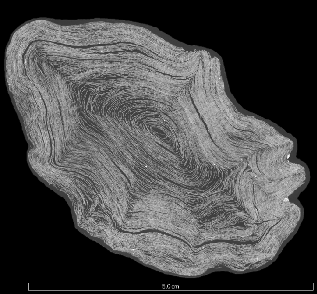
The subtle differences that distinguish ink from papyrus must be teased out of data like this.
The compressed-region problem
For as long as we’ve been working on these scans, it’s been apparent that some regions of a scroll look worse than the resolution used to scan them would suggest. These crops come out blurred, foggy, "compressed" — papyrus layers that should be cleanly separable become hard to tell apart. When panning through layers, the sheets could almost be seen “behind” this fog. Recent scanning experiments conducted at very high resolutions (0.55 µm detector pixel size) have finally given us an answer to the question of why these areas exist.
The explanation starts at the fiber level. Carbonized papyrus fibers contain small internal cavities and tubular structures, and when many of them pack together densely, these microscopic structures disturb the X-ray beam enough to deviate it a little bit. This effect results into a local haze-like degradation in the scan. The likely culprit is the carbon itself: carbonized fibers are probably close to graphite, and graphite is a strong decoherer — a material that scrambles the X-ray wavefront rather than passing it through cleanly. The effect is worst in the most densely packed regions, where many fibers contribute to the haze at once.
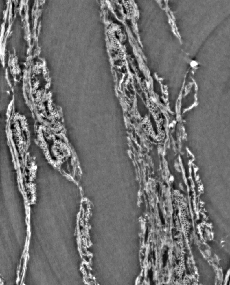
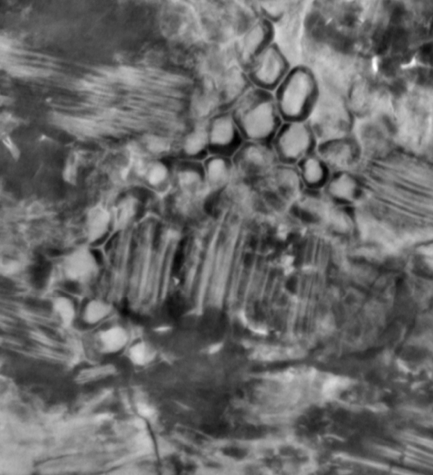
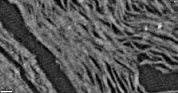
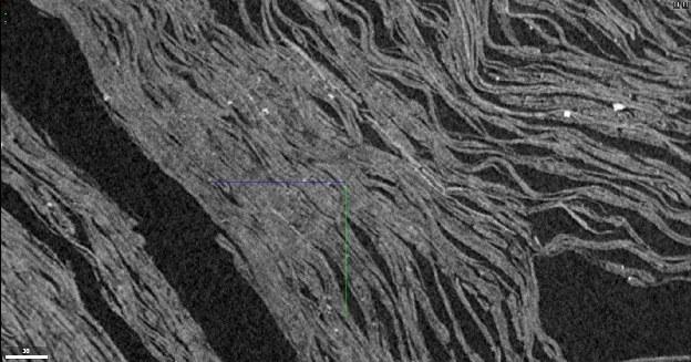
The difficulty of unwrapping scrolls begins here. Blur the boundaries in the scan, and every downstream step gets harder: surface localization (finding the writing surface within the volume) turns noisier, mesh tracing turns less stable, and ink recovery may miss information it needs.
The main point is that scan quality is local. A scan can hold excellent regions and nearly-impossible-to-unwrap ones in the very same volume.
Three coupled scan parameters
Scanning is controlled by several parameters, but three are especially important:
| Parameter | Meaning | Why it matters |
|---|---|---|
| Voxel size | The physical size represented by each voxel in the reconstructed 3D volume. | Smaller voxels can preserve finer structures, but increase scan time, reconstruction hardships, and data size. |
| X-ray energy | The energy of the X-rays used for imaging. | Energy affects penetration, contrast, phase behavior. |
| Sample–detector distance | The distance between the scroll and the detector after X-rays pass through the object. | This controls how phase shifts develop fringes before detection. |
To understand why the third parameter matters, we must explain phase contrast.
X-rays behave like waves. Passing through a material doesn't just absorb them; it also shifts their phase. Different shifts can be induced by different refractive indices of materials in the sample. As the wave-front travels away from the sample and towards the detector, it interferes with itself, generating interference fringes at the detector corresponding to the position where the accumulation of shift in phase started or ended: interface boundaries. The fringes act as a natural “edge enhancement”, and this effect is known as phase contrast. In objects with very little attenuation contrast – like our scrolls – this can be especially useful. A computational step called phase retrieval can turn those phase contrast fringes into a higher-contrast reconstruction; the Paganin algorithm is one commonly used method for it.
But more phase contrast isn't always better. Push sample-to-detector propagation distance (a knob that usually is tuned to optimize phase contrast) too far and the same effect can turn against you, blurring the volume and reducing clarity rather than contributing to it.
The scanning problem is a balance:
- enough phase contribution to reveal useful structure;
- not so much that the scan becomes dominated by haze or decohesion;
- enough X-ray energy to penetrate the object and separate layers;
- not so much that useful absorption contrast disappears;
- and voxels small enough to resolve the structures that matter, without shrinking so far that scanning a full scroll stops being practical.
For recent full-scroll scans (ESRF/BM18), a practical regime has been around 2.4 µm isotropic voxels, 22 cm propagation distance, and about 78 keV average incident energy. This isn't a universal recipe. Scrolls which are very large or very small may benefit from some tweaks, but we’ve found that this recipe works well in the samples we have scanned to date. We scanned many samples with a lower resolution configuration which seemed to be "optimal" (but not as good as the first): around 9 µm isotropic voxels, 1.2 m propagation distance, and about 110 keV average incident energy.
Why resolution helps, but does not solve everything
The most reliable direction so far has been to reduce voxel size. Smaller voxels help in several ways:
- they preserve finer papyrus structure;
- they are less affected by the beam decohesion (haze);
- they reduce ambiguity between adjacent layers;
- they may preserve more of the ink-related morphology;
- they induce cleaner absorption and phase contrast.
Given these benefits, it seems fair to ask “why not just scan everything at the highest possible resolution?”
The curse of dimensionality is why. Perhaps counterintuitively (for those not familiar with 3D volumes) if voxel size is halved in each dimension, you might think the number of voxels is simply doubled, but in actuality it is eight times the voxel count for the same physical volume! As an example, moving from 8 µm to 2 µm is not a 4× data increase; it is roughly a 64× increase. Moving toward 1 µm for a whole scroll becomes a data, scan-time, motion, and beamline problem.
Small regions can be scanned at higher resolution. Full scrolls cannot yet be scanned everywhere at sub-micron resolution in a practical production workflow.
Current failures have to be read carefully. Ink not recovered from a scroll doesn't necessarily mean the signal isn't there. It may be absent, or it may be present but not yet exploitable by the current surface placement, labels, model architecture, or training data. Right now we do not always know which part of the pipeline is limiting us and the limiting factor is to be assessed on a scroll-by-scroll basis.
Some regions leave the scanner already degraded: densely compressed papyrus scatters the beam into haze that no downstream algorithm may fully undo — and scanning whole scrolls at sub-micron resolution is not yet practical. When ink fails to appear, we do not always know which part of the pipeline is limiting us; the limiting factor has to be assessed scroll by scroll.
2. Unwrapping: turning disconnected voxels into a surface
After scanning, we have voxels, packed together into a volume – a large 3D cuboid. The volume is a sort of 3D photo: it does not tell us which voxels belong to the same sheet. It does not tell us where one wrap — one full revolution of the papyrus around the roll — ends and another begins. It does not provide a graph of connectivity. And it does not tell us whether two distant points are part of the same papyrus layer. (This post uses "wrap," "winding," "sheet," and "layer" more or less interchangeably for the same idea: one continuous turn of the papyrus as it spirals from the outside of the roll toward the center.)
So the first step in unwrapping a scroll is surface localization – finding the writing surface inside a 3D voxel volume.
Surface prediction
A common starting point for surface localization is semantic segmentation: assigning a class label to every voxel — either it’s the recto surface of the papyrus, or the “background”. However, a model trained this way doesn't hand back a finished scroll surface. It outputs a dense 3D prediction that later steps can use as geometric cues.
In papyrus terminology, two sides of a sheet are often distinguished. The recto is the written surface, its fibers running horizontally, and it's always rolled facing inward, toward the center of the scroll. The verso is the back of the papyrus, where the fibers run vertically instead.
The architecture usually chosen for this job is a 3D U-Net. The model learns local and contextual patterns in the CT data and produces a voxelwise surface probability.
Two checkpoints built on this idea anchor the current pipeline: surface_recto_3dunet, a checkpoint for the recto-surface predictor (recto — the papyrus's written surface, defined below) used in the pipeline behind the project's technical paper (see References); and surface_m7_nnunet, the nnU-Net ("m7") component — nnU-Net is defined just below — of the 1st-place solution to the Kaggle competition described below.
Surface prediction was the subject of a dedicated Kaggle competition, "Vesuvius Challenge – Surface Detection," with a $200,000 prize pool in November 2025. The competition's scoring metric was deliberately topology-aware rather than voxel-accuracy-based: it rewarded connected, gap-free predictions and penalized exactly the failure modes described later in this section — holes, mergers, and sheet switches — rather than treating them as small per-voxel errors. The winning approaches converged on nnU-Net, a self-configuring 3D U-Net framework that automatically adapts its own architecture and training pipeline to a given dataset's geometry and voxel spacing, instead of requiring a human to hand-tune it.
Here's the winning recipe condensed to a single sentence: take an off-the-shelf nnU-Net model configured for a couple of patch sizes, train it for a very long time (well over the default 1,000 epochs), and average their predictions together (a process known as ensembling).
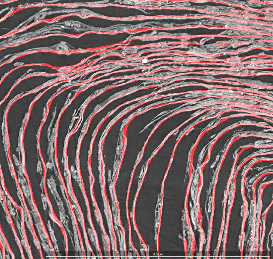
Create datasets with labels better localized on the papyrus’ recto or train ML models that can better preserve the sheets’ topology in the predictions. The open question is reaching a high level of topologic accuracy in densely packed regions, regions affected by high curvature or in spots where the papyrus is damaged. Different representations are also worth investigating, like using a Distance Transform rather than a Binary Segmentation (e.g. https://www.kaggle.com/competitions/vesuvius-challenge-surface-detection/writeups/5th-place-solution)
Surface predictions are useful, but they are not usable as the final geometry for unwrapping. Dense predictions often contain holes, local deviations, false positives, or accidental mergers between nearby layers. In a normal image/volume segmentation task, a small local error may be tolerable. Here, a small local error can send a traced mesh onto the wrong wrap entirely, with no easy way to recover.
Finally, to virtually unwrap the localized surface, we need to represent it explicitly as a mesh.
Meshes: adding connectivity
The purpose of the meshing step is to determine the geometrical connectivity of the scroll. It supplies the necessary information we cannot recover from the voxel grid alone: the ability to say "this point is next to that point, on the same surface."
The current workflow uses surface predictions as guidance, then builds or refines explicit meshes that can be inspected and corrected.
Imagine trying to follow a trail which is not well defined. It’s difficult to see where it continues in the forward direction. It has many areas in which you’re not sure whether it continues left, right, or some other direction. This is the type of path given by surface predictions. The mesh is then a map of the path you’ve chosen to take, whether right or wrong. If the map is wrong in one place, you’ll end up off-course, and it may be difficult to find the correct path to recover.
The areas we most often see this type of problem are:
- mergers, where two nearby sheets are joined by mistake;
- holes, where the predicted surface disappears;
- sheet switches, where a traced mesh jumps from the intended sheet to a neighboring wrap;
- compressed regions, where the image itself gives weak or ambiguous evidence;
- damaged regions, where the physical papyrus is torn, folded, or missing.
These errors determine whether a flattened rendering shows a coherent writing surface or a corrupted one. We greatly value community contributions that help us trace sheets more accurately, avoiding these failure cases.
If you know geometry processing, optimization algorithms, or C++, this is one of the highest-leverage places to contribute. Many errors in the surface predictions can be fixed during or mitigated during the meshing step with either subsequent optimization or post-processing algorithms. Community contributions building alternative, scalable meshing algorithms that attack the current failure modes are encouraged (e.g. github.com/Hob3rMallow/scrollfiesta_public)
Surface mesh representations
The unwrapping software used by our team, VC3D, uses a custom format called 'tifxyz,' an alternative to widely-used 3D formats such as .obj or .stl. Its key benefit is that it enforces grid topology on the surface mesh — meaning, again, a single flat sheet. The flat coordinate system on the surface is carried explicitly exploiting a 2D grid structure. Indeed, the surface mesh (QuadSurface in the C++ code; Tifxyz in Python, via vesuvius.tifxyz.Tifxyz/read_tifxyz()) is represented by a 2D array of 3D vertex coordinates: the array's shape determines the mesh's grid structure, and the vertices define its actual shape in space. That grid of coordinates is saved as three separate TIFF images, one each for x, y, and z coordinates (as float32). The format can also mark a given cell as missing, either by setting each coordinate to -1 or via an optional sidecar mask image. Converter scripts move between tifxyz and .obj in both directions (vc_tifxyz2obj, vc_obj2tifxyz); going from .obj to tifxyz requires an accompanying .griduv sidecar file specifying the intended grid structure (a legacy converter without this requirement also exists, but is not recommended for new work). The core representation itself lives in QuadSurface.cpp.
Visualizing a mesh
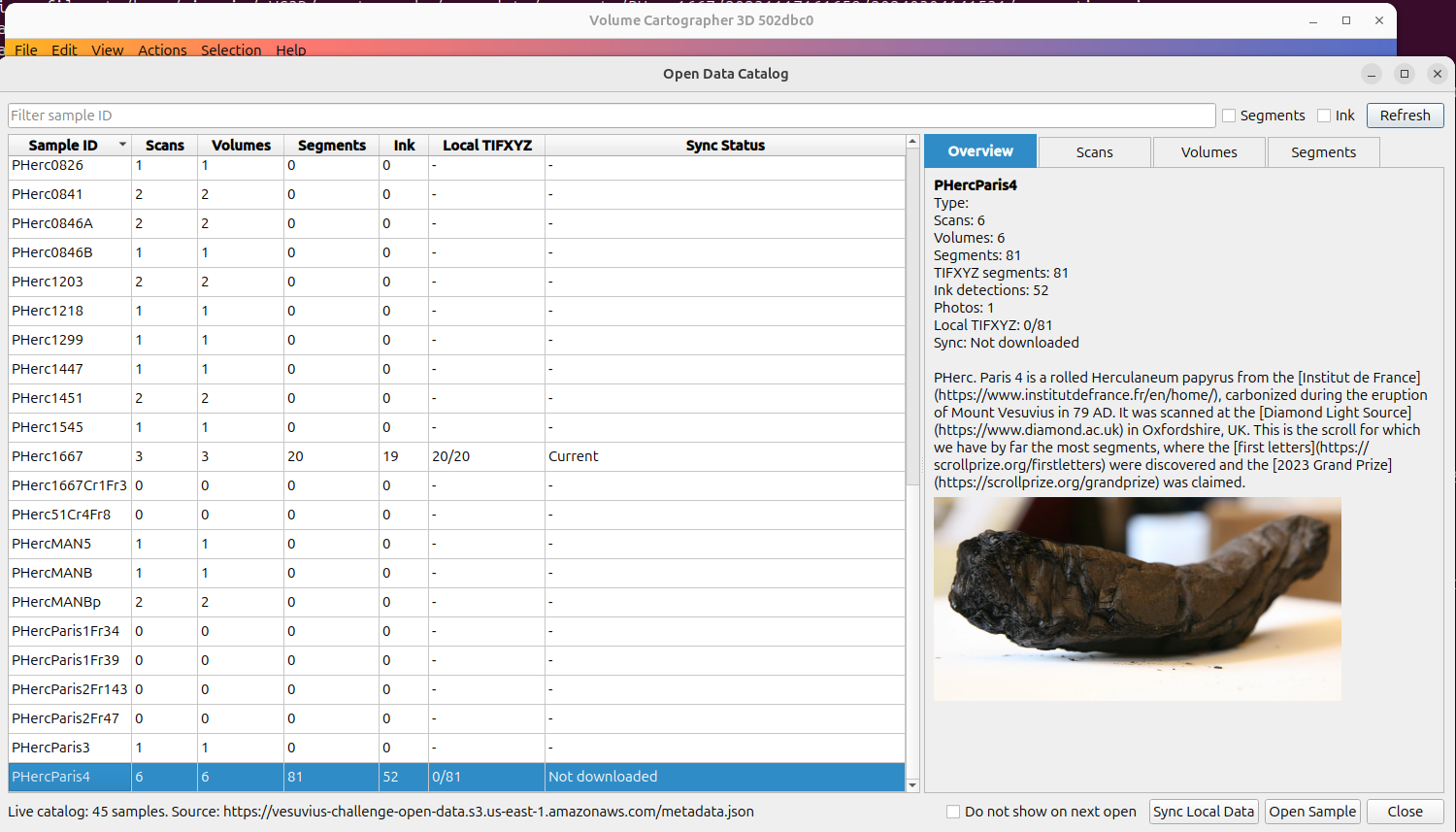
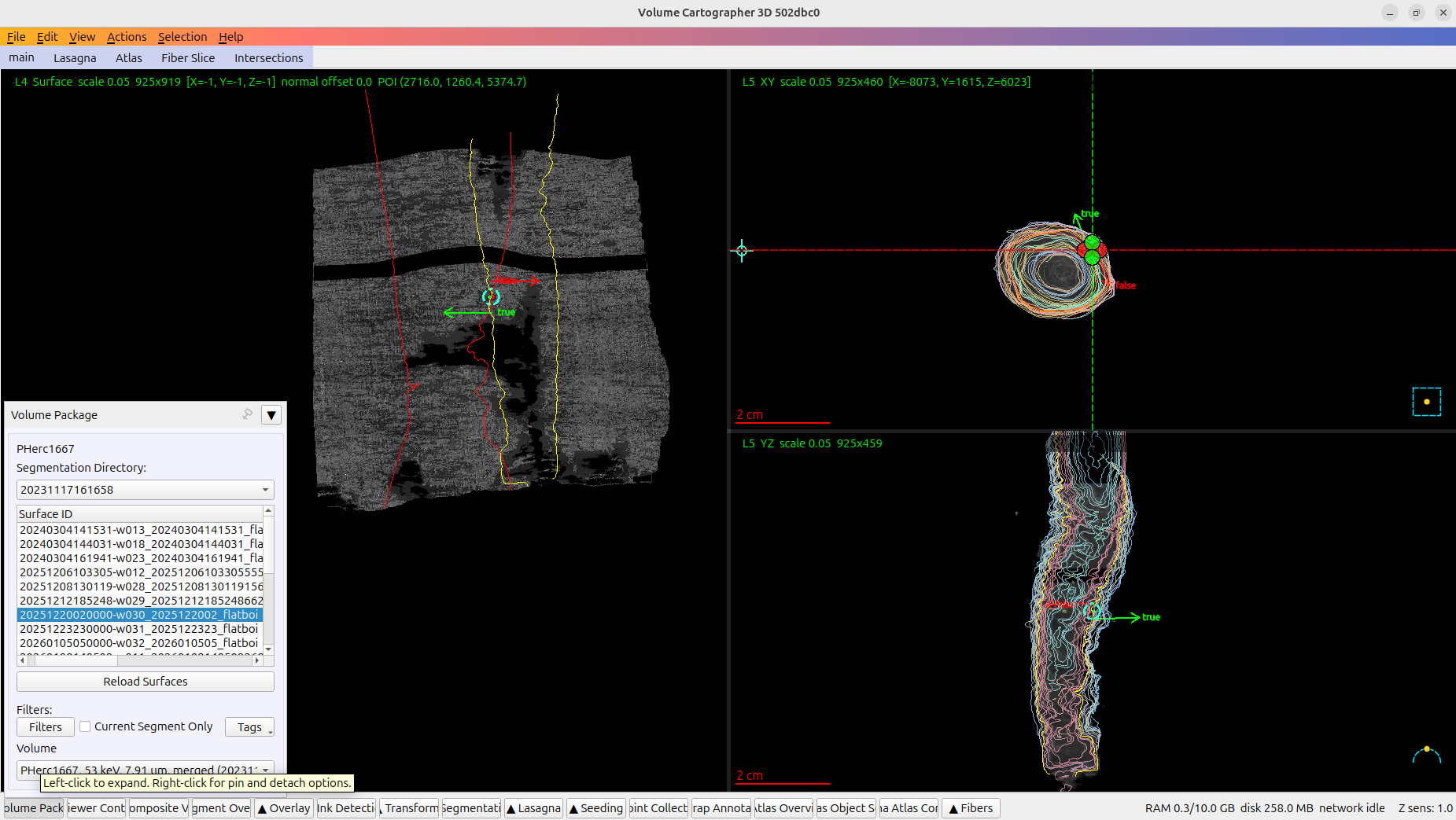
VC3D makes it possible to visualize the CT scans, meshes, and annotations all in one tool. The CT data for the large scrolls, which can reach dozens of terabytes, is streamed remotely and synchronized from the S3 Open Data bucket, generously provided to the project by AWS. A hands-on VC3D tutorial walks through installing the software, loading scroll data, and annotating fibers and windings.
Normal grids, GrowPatch, and local tracing
We have several different tools that all attack the same underlying task — turning a surface prediction into a trustworthy mesh — with different tradeoffs between speed, automation, and reliability.
To trace a surface VC3D produces meshes (internally can be called also 'patches') based on a recto surface prediction volume, i.e. a volume produced by a surface segmentation model that is '1' everywhere that's on the papyrus surface.
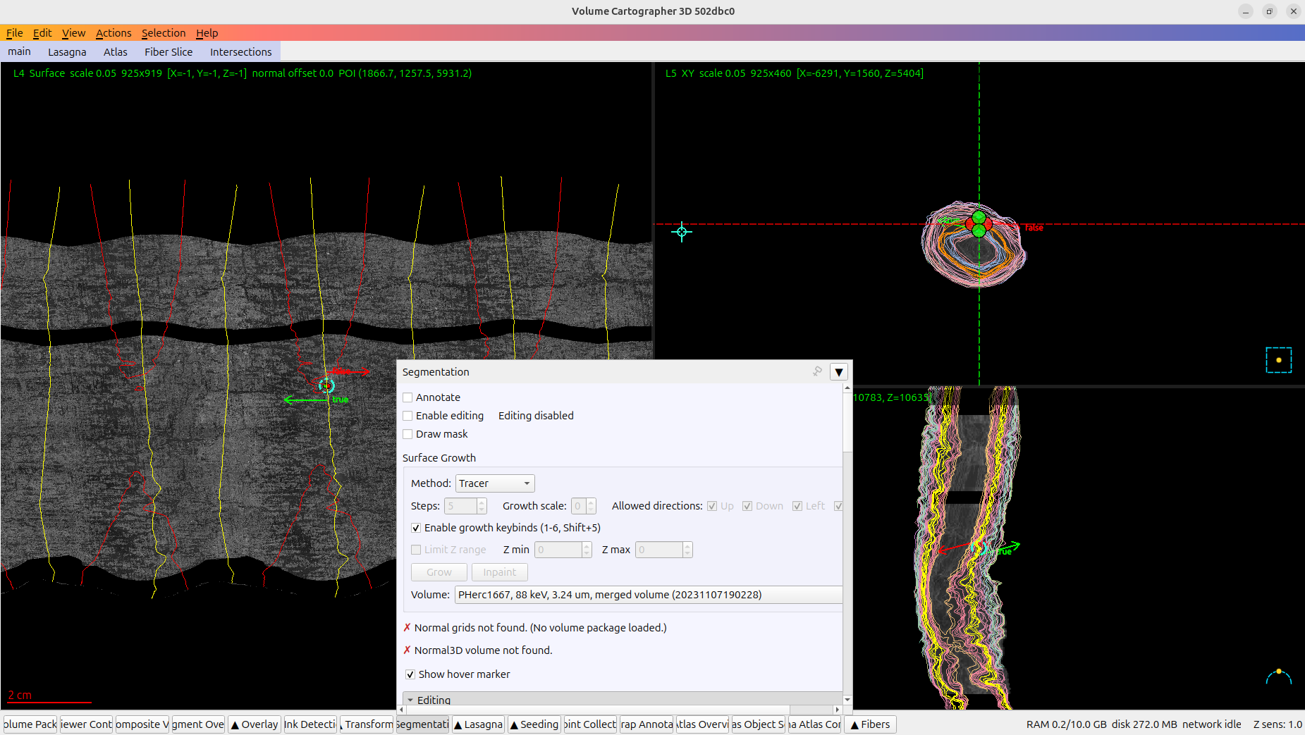
VC3D needs local orientation information to trace surfaces well. A normal is simply a vector perpendicular to a surface — for a papyrus sheet, that means it points straight "out of" the sheet. Stack a coarse 3D field of these local orientations together and you get a normal grid, which helps guide mesh growth. A dedicated tool, vc_gen_normalgrids, generates, converts, and builds resolution pyramids of these normal grids from the CT volume.
The workflow can then use routines such as GrowPatch. A GrowPatch-style routine starts from a seed point or an existing patch and extends a local mesh along the predicted surface. Recall the trail discussed in the previous section. GrowPatch attempts to follow this trail, iteratively. Mathematically, this means optimizing concurrently for a combination of objectives: to follow the predicted papyrus surface, keep the local geometry smooth, hold mesh spacing to something reasonable, follow whatever local orientation evidence is available, and resist the pull of a nearby sheet it could easily jump onto instead.
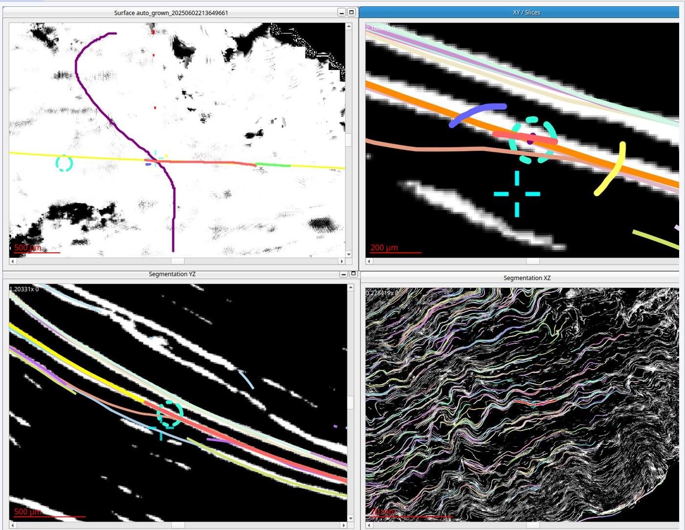
This works well when the prediction is clean and the layers are separable. But it fails when the prediction topology does not match the real papyrus topology (e.g. because some predicted sheets incorrectly merge in the surface prediction volume). In practice, automatic growth still needs human inspection and correction.
The current system is therefore best described as semi-automated.
Copy Out/In: exploiting neighboring wraps
Once one wrap has been traced well, nearby wraps further in or out may have similar local curvature. The Copy Out/In workflow exploits that fact. It uses an existing mesh as a geometric reference and tries to transfer or offset the tracing to a neighboring layer, implemented in vc_grow_seg_from_seed.cpp and GrowPatch.cpp.
This is powerful because adjacent wraps often resemble each other. But it is also risky: if the source mesh contains a local error, that error can propagate. So Copy Out/In is useful as an acceleration tool, not as an unchecked replacement for validation.
A "neural" learnt version of the copy out/in also exists, implemented in infer_rowcol_triplet_wraps.py and released as the copy_displacement_latest checkpoint on Hugging Face (trained on 2.4 µm data downscaled once → 4.8 µm).
This method is exposed in the VC3D interface through a dedicated Neural Tracer panel. A baseline checkpoint, ps256_copy_baseline, is also available for comparison against the actively used copy_displacement_latest, and the panel itself is implemented in SegmentationNeuralTracerPanel.cpp.
Lasagna: smoother optimization of one or more sheets
The lasagna is an alternative to GrowPatch and copy out/in. It provides a more flexible optimization framework for solving the same problem of creating surface meshes semi-automatically. It can better fit complex, curved regions of the scroll, at the expense of being somewhat more computationally intensive.
The lasagna can (optionally) optimize several stacked sheets at the same time, so they are all consistent with each other; as such it can be used similarly to GrowPatch followed by copy out/in. Other modes include making local corrections so a 'draft' surface is moved closer to the true surface while keeping certain points fixed. In all cases, surfaces (represented as a stack of non-intersecting quad-meshes — quad-faced grids of vertices, more on why below) are iteratively adjusted to agree with prediction volumes as closely as possible, and also with user-provided 'correction points' that define locations known to be on the papyrus surface.
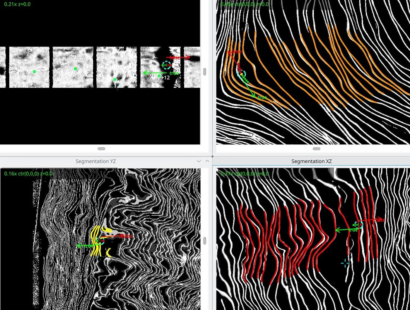
The lasagna needs richer prediction volumes than a plain recto surface prediction can offer: a dense normal volume predicted by a U-Net, and a surface density (called 'gradient magnitude') volume that represents how closely spaced the papyrus windings are. The second one works like this: a second U-Net predicts a fractional winding position field for every voxel — essentially "how much further out in the scroll do we get, moving from one side of this voxel to the other point, expressed as a fraction of one full winding." That field is built from distance transforms to sheet skeletons, then normalized into a monotone field via iterative weighted averaging. Gradient magnitude tells how fast winding position changes as you move through space. Integrate this along a short strip between two points and you get the number of windings crossed to go from one to the other — which is why it doubles as a proxy for winding spacing. High gradient magnitude means sheets are packed tightly together locally; low means they're far apart.
Technically, the lasagna can do a global optimization of the entire local surface (or surfaces), implemented using PyTorch. GrowPatch, by contrast, uses Ceres — a classical nonlinear least-squares solver of the kind widely used in robotics and computer vision — inside an iterative growth loop that adds quads progressively and repeatedly re-optimizes an outer fringe.
The predicted volumes (normals, etc.) that are used as input to the main lasagna surface optimization can also be used to trace fibers, i.e. to semi-automatically follow the lines of papyrus fibers through the 3D volume, given sparse human-specified keypoints.
The full lasagna codebase lives at github.com/ScrollPrize/villa/tree/main/lasagna.
2D Parameterization and Flattening
Flattening takes each point on the 3D mesh and assigns it a 2D coordinate. The same trick as making a flat map from a curved globe, but in our case we are aiming to preserve local distances as much as possible: we are looking for a transformation from 3D -> 2D which is isometric.
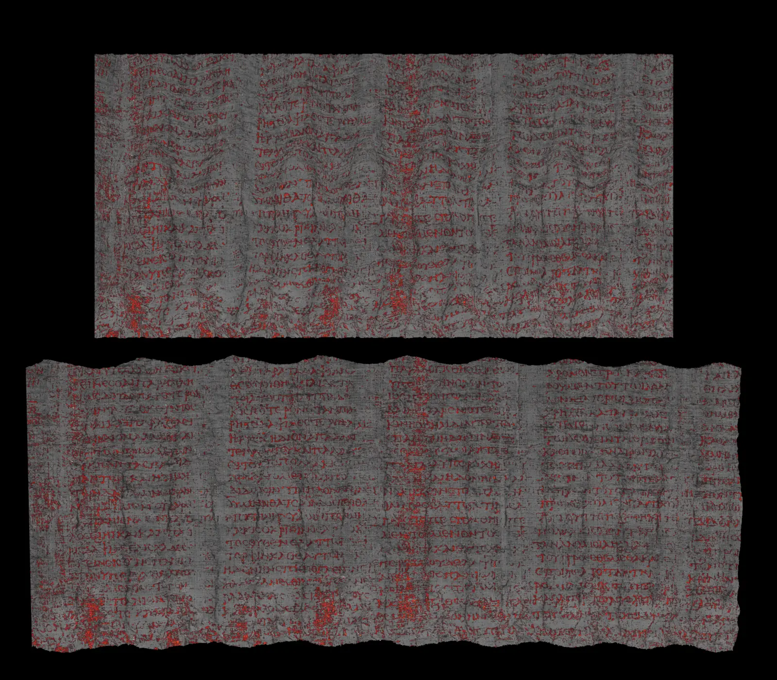
VC3D's current production flattening tool is flatboi, which uses SLIM (Scalable Locally Injective Mappings), minimizing the Symmetric Dirichlet Energy (which is small the lower the isometric distortion induced by the map).
Fibers as connectivity clues
Papyrus is made of fibers. These fibers carry geometric information.
If you recall from the flattening step, to get a mapping from 3D space to 2D space, we can map our 3D points in rows and columns in the correct order (preserving distances) – in the parameterized space these rows and columns “axes” are usually called U and V. Conveniently, a papyrus sheet has these axis “physically” defined! Within each sheet are vascular bundles oriented vertically or horizontally and each one – if perfectly segmented – could be used directly as an individual row or column. Amazing! The papyrus sheet itself is providing a direct way to parametrize its surface!
If we can manage to trace the fibers, we can directly obtain oriented axes in the papyrus. This information can not only help us to flatten the segmented sheets, but also to segment the surface itself! Unfortunately, if you recall the Scanning section, beam decohesion on fibers is also what makes the volume blurrier. So fibers can be both a blessing and a curse.
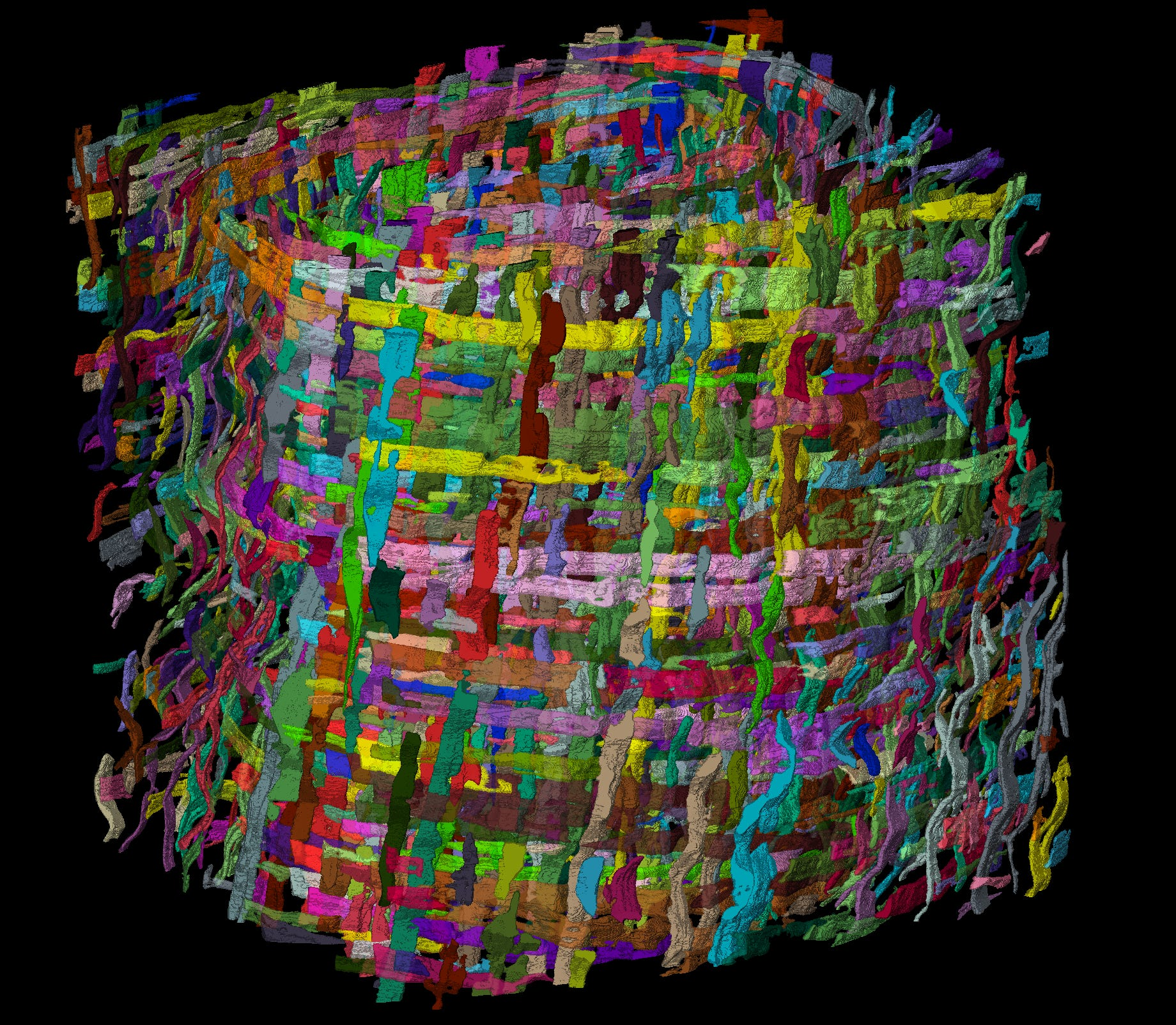
The crossing horizontal and vertical bundles physically define the row-and-column (U and V) axes that can parameterize the sheet’s surface.
In VC3D we have a fiber tracer tool, which is part of the Lasagna optimization ecosystem. It is not fully automated, and the line annotation widget inside VC3D is what drives it. Once fibers are annotated, atlas.py can pair fibers / skeleton annotations and optimize a “patch” through them.
This is not the only way to trace fibers. Some of the project's most valuable fiber-skeleton labels were traced by hand years ago in WebKnossos (a web-based tool for tracing and annotating skeleton-like structures voxel by voxel in large volumetric datasets), against older EduceLab-era scans taken at Diamond Light Source, a synchrotron facility distinct from ESRF — the facility behind the more recent scans discussed throughout this post.
These annotations were voxelized and used to train a semantic segmentation model for fibers. We provide a checkpoint named fiber_hz_vt — weights of an nnUNet model trained on "horizontal/vertical" fibers manually traced by annotators on the older 7.91 µm scans.
Since we rescanned some of the old scrolls with the new protocol at ESRF, it can be important to match both labels and predictions.
With cross-frame training we can work with volumes that live in different coordinate frames at once, bridged by an affine transform — a combination of rotation, scaling, and translation. A new dataset class, CrossFrameZarrDataset (cross_frame_dataset.py), does so using a transform.json sidecar file that records the map between the old annotation's frame and the new scan's.
The main problem is obtaining, either through direct tracing or through semantic/instance segmentation, a way to identify and separate long fibers with the right connectivity. The same problem is shared in connectomics — the field that reconstructs a brain's wiring diagram by tracing individual axons and dendrites through teravoxel-scale 3D electron-microscopy volumes.
If you know classical computer vision or point tracking techniques, robust fiber tracing is exactly this kind of problem. The goal should be reliable connections — a tracer that confidently follows fewer fibers correctly is more useful than one that follows more fibers with a higher error rate.
Spiral fit: a global prior
Local tracing can drift. Fibers can help, but they are also local or semi-local. There is another source of information: the scroll was originally a spiral.
Call it a prior: an assumption used to guide a reconstruction. Here, it's that before damage and carbonization, the papyrus was rolled into a roughly cylindrical spiral. The real scroll is damaged, compressed, and deformed — but it's not an arbitrary tangle.
A spiral fit starts from an idealized spiral and deforms it to match evidence from the scan, and that evidence can come from almost anywhere else in the pipeline: traced patches (small parts of the surface produced by GrowPatch or lasagna), fiber skeletons (created semi-manually using the lasagna workflow), surface prediction skeletons (automatically derived from the surface prediction volume), point constraints (e.g. "these points are one winding apart", "this patch is on winding 20", "these points are on the same surface"), and normal fields (the same dense normal-prediction volumes the lasagna produces, described above).
Each of these sources of information provides a hard (verified) or soft (unverified) constraint on where the spiral windings should be. The spiral tries to satisfy as many of these constraints as possible, deforming the spiral as needed, and preferring the hard constraints.
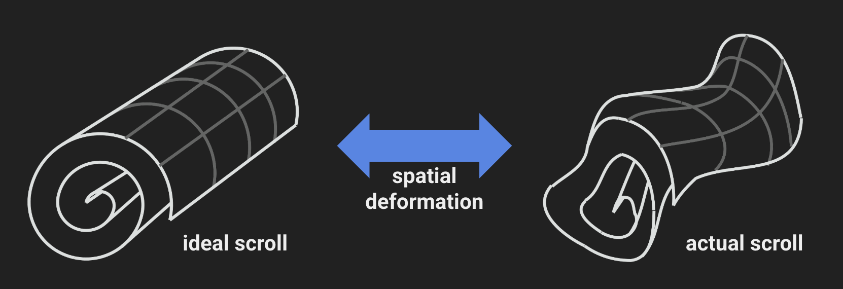
One way to represent the deformation is through a stationary velocity field. In simple terms, this is a smooth 3D field that tells points how to move from the ideal spiral toward the observed scroll. If the transformation is smooth and does not tear or fold the coordinate system onto itself, it preserves the global structure of the spiral while still adapting to damage. The fitting process itself is implemented in fit_spiral.py, and there is a full tutorial on running it.
A global prior can organize and regularize geometry, allowing a single consistent result to be produced from disconnected annotations, bridging small gaps and interpolating windings. But where annotations are sparse or the volume is highly ambiguous, spiral fitting is still under-constrained, and won't necessarily follow the true sheet surfaces.
Devise better evaluation suites and loss functions to fit the spiral. Increase its expressivity and reduce the number of needed annotations. Most importantly, relative winding number annotations seem to have a great impact on the spiral fit. Automating these procedures will boost scalability by a great extent!
Label quality: one of the main unwrapping bottlenecks
Machine learning needs labels. For surface models, those labels often come from human-generated meshes or annotations — enormously valuable, but approximate. They may wiggle. They may drift slightly off the true surface. They may avoid the most ambiguous regions. This is also valid for manually or semi-automatically traced fibers. They may represent the best usable tracing rather than exact truth.
This creates a subtle problem: the model isn't always learning the physical feature itself. It's learning from an imperfect representation of that feature.
Why did we move forward with these datasets instead of fixing them first? The labels were not bad; they were good enough to support major progress in the previous phase of the project. However, as the pipeline becomes more ambitious, label quality has started to become one of the limiting factors.
No method yet traces a complete, correct surface through a scroll automatically — and the labels used to train surface models are themselves approximate. The model isn't always learning the physical feature itself, but an imperfect representation of it: label quality is now one of the main unwrapping bottlenecks.
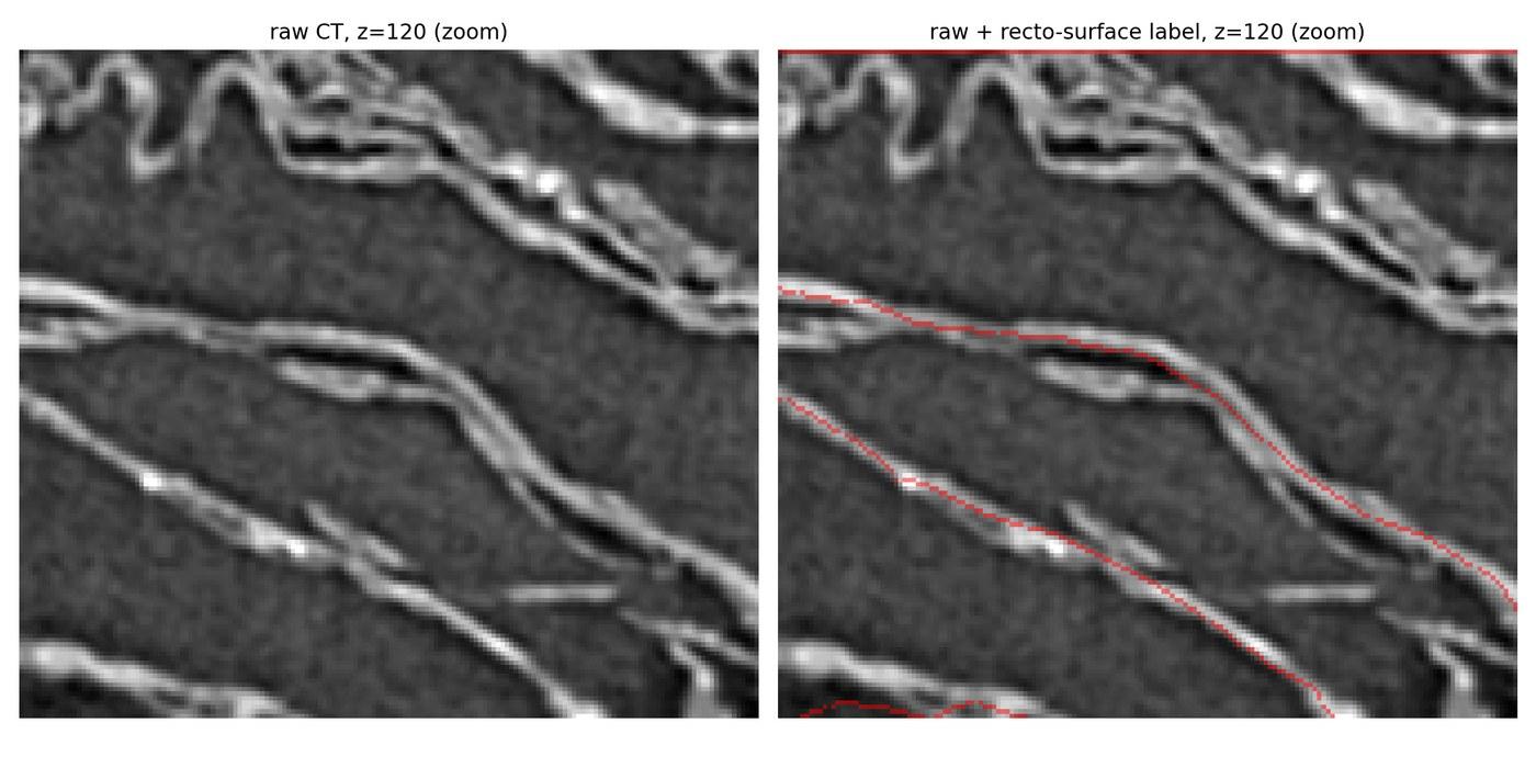
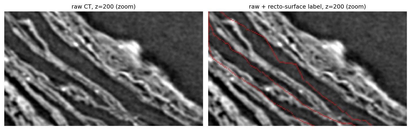
A useful direction is label snapping: using the raw CT signal and local geometry to move approximate labels back onto the most plausible papyrus surface / fiber. Another direction is active learning, where the model identifies the most uncertain or valuable regions and asks humans to correct only those.
If you have experience with 3D annotation, active learning, or data-quality workflows, this is a place where careful, small-scale work can matter more than scale. The next major gains in unrolling may come from better labels rather than simply larger models — a smaller set of precise labels in hard regions may be more useful than a larger set of approximate labels in easy regions.
3. Ink recovery: reading the scrolls
Once the surface is traced and flattened, the next question is: where is the ink?
The phrase ink detection is widely used, but there are two related tasks:
- Ink detection: decide whether ink is present in a region.
- Ink segmentation: locate the ink precisely, ideally in 3D.
For an ideal pipeline, ink segmentation is the cleaner target. We would like to say: these voxels correspond to ink, these do not. But usually, the ink signal is too subtle for direct voxel-level annotation. That is why the current pipeline often uses models that work on surface-conditioned renders (also called surface volumes).
A surface-conditioned render, or a surface volume, is a flattened 3D subvolume centered on a segmented sheet surface. Using the mesh’s 2D flattened coordinates, each point on the sheet is mapped back into the original CT volume. The center layer corresponds to the sheet surface, while additional layers are sampled at positive and negative voxel offsets along the local surface normal. This produces an image stack where the curved papyrus surface is represented as a flat layer, making nearby material and possible ink easier to inspect or process.
Fragment-trained ink models
Detached fragments are pieces of scroll where the writing surface is exposed. Some of these fragments exist because early researchers tried to physically open sealed Herculaneum scrolls: starting in the 1750s, first with Antonio Piaggio's mechanical unrolling device — a frame of weights and silk threads — and later with a range of chemical treatments, gas exposure, and slicing. These methods often cracked or shattered a scroll; some survived well enough to be read this way, many others were damaged or destroyed outright. Because the ink on a detached fragment's exposed surface is visible, the fragment can be photographed, often with infrared imaging. The same fragment can also be CT-scanned.
That creates a training pair:
- input: CT data around the papyrus surface;
- label: visible ink from the photograph.
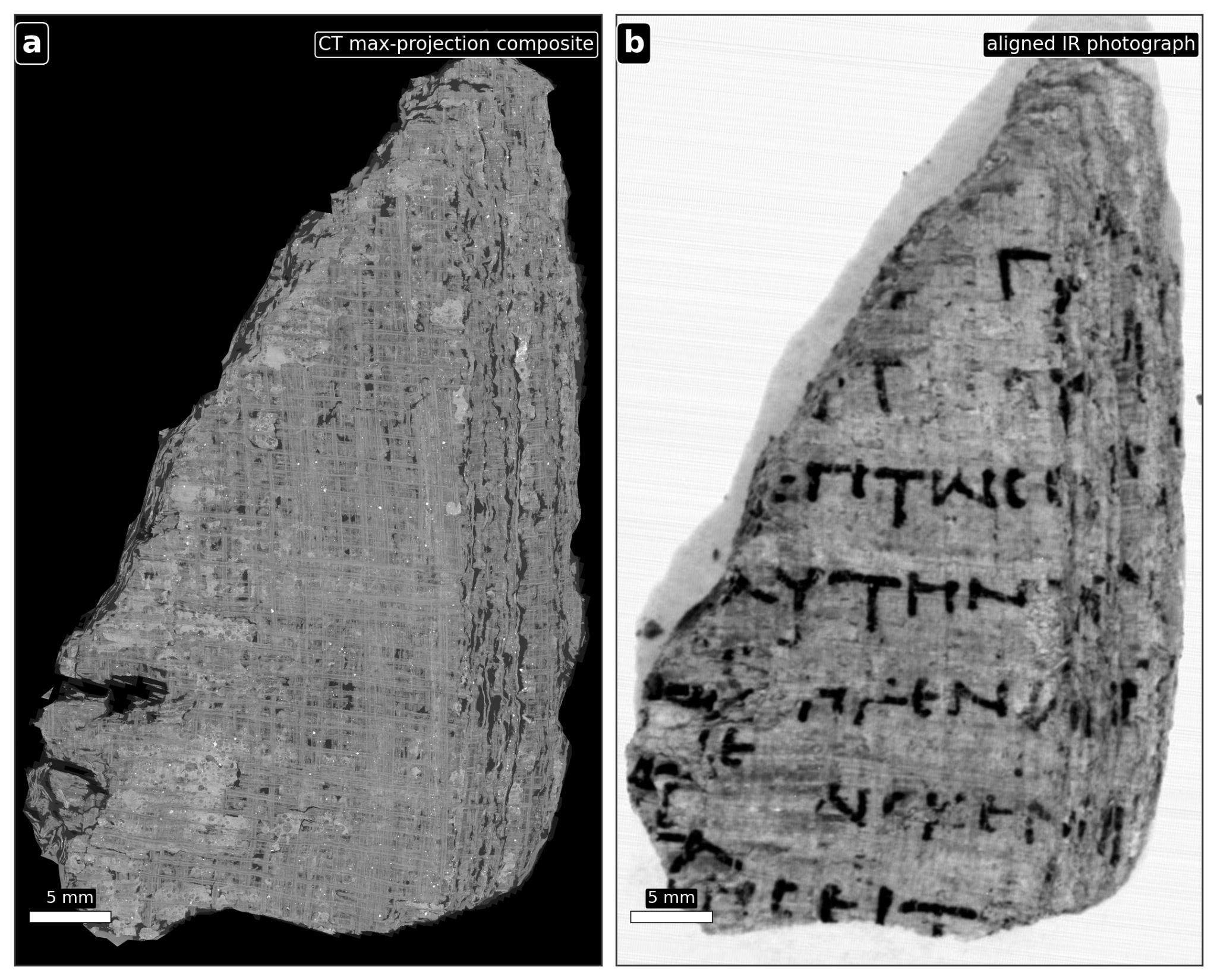
The model learns from fragments and is then applied to sealed scrolls. Generalization is not straightforward!
Working on surface-conditioned renders of the fragments’ outer sheet, the model receives a local 3D neighborhood and predicts a 2D ink probability map on the flattened surface.
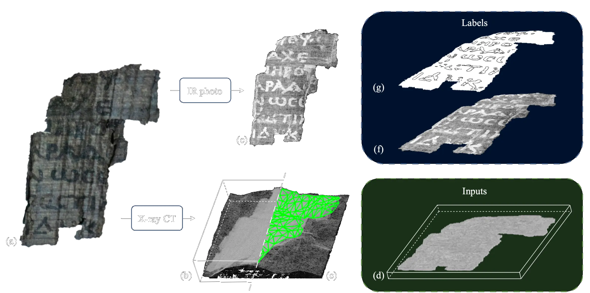
However, fragment labels are 2D: the photograph tells us where ink appears on the exposed surface, but not exactly where the ink signal sits in depth inside the CT volume.
The model is not OCR. It is not given Greek words, transcriptions, dictionaries, or language-model targets. It learns local CT texture and morphology associated with ink labels.
Pseudo-labeling: bootstrapping weak signals
Sometimes a fragment-trained model reveals faint but coherent ink traces inside a sealed scroll. When that happens, one can create pseudo-labels.
A pseudo-label is a provisional label created from model output and human review rather than direct photographic ground truth. The loop is:
- Train on fragments.
- Run the model on a sealed scroll.
- Identify plausible ink traces.
- Create conservative pseudo-labels.
- Fine-tune the model.
- Run inference again.
- Repeat.
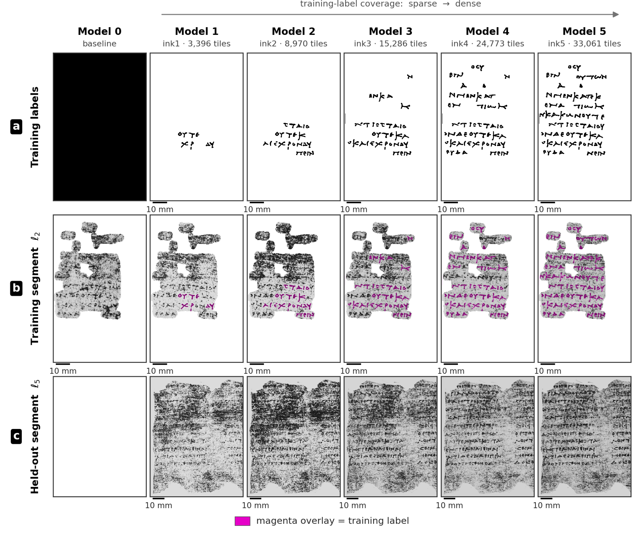
Row (a) shows the training labels, row (b) predictions on a training segment (magenta = training label), and row (c) predictions on a held-out segment, which grow steadily cleaner and more legible.
A concrete record of this loop exists in the six PHerc.1667-iteration-0 through -5 checkpoints released alongside the project. Each of the six shares an identical architecture (a ResNet3D-50 backbone initialized from Kinetics-700 weights, feeding a 2D U-Net decoder) and an identical training budget, differing only in how much pseudo-labeled data it was fine-tuned on — from a cross-segment baseline at iteration 0 up to the densest available label set at iteration 5. Why initialize from a video dataset? A video clip and a CT volume are both fundamentally 3D data — two spatial axes plus a third (time for one, depth for the other) — so a 3D-convolutional network pretrained on one transfers surprisingly well to the other. All six checkpoints are released on Hugging Face: iteration-0, iteration-1, iteration-2, iteration-3, iteration-4, and iteration-5.
This process helped recover readable text in PHerc. 1667. But it is not guaranteed to work everywhere. In some scrolls, predictions improve and then plateau. In others, current models show little or no convincing ink.
The current ink detection model, which works on 2.4 µm data, is https://huggingface.co/scrollprize/ink_canonical_2um, inference code: https://github.com/ScrollPrize/villa/tree/main/ink-detection/optimized_inference
We have evidence that working on 1.1 µm data yields cleaner results than 2.4 µm data. But scanning at high resolution is impractical.
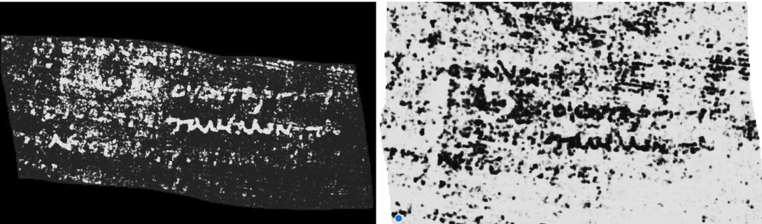
]οὐδὲ γὰρ
]τὰ μέλλοντα τελεῖϲθαι πρ[
The square brackets follow classics and papyrology's standard "Leiden Convention" for transcribing damaged text: they mark text that is missing or illegible at that point in the original, not a typo or a transcriber giving up. An open bracket with nothing closing it, as in "πρ[", means the word is simply cut off there by damage.
What happens if the models don’t generalize? The right conclusion here is neither "the scan failed" nor "the model failed." At the moment, several explanations remain possible:
- the scan may not capture the relevant signal strongly enough;
- the surface may be slightly misplaced (suboptimally localized);
- the ink labels may not match the true location of the ink signal;
- the model architecture may not be exploiting the right features;
- the ink morphology or chemistry may differ across scrolls;
- the signal may be present but below the current pipeline's ability to use it.
This is why better diagnostics matter just as much as better models — without them, it's hard to know which of these failure modes you're even fighting.
4. Data scale: the infrastructure bottleneck
A full-resolution scroll volume is huge — too huge to just download to a laptop and work with as a local folder. So the project increasingly depends on chunked, cloud-friendly formats instead.
One important format is OME-Zarr, which stores large multidimensional arrays in chunks and often at multiple resolutions, letting software read only the region it needs rather than loading an entire scroll.
Getting the data format right turns out to matter as much as the algorithms built on top of it, because it determines what research is practical at all. A model that requires copying tens of terabytes locally shuts most contributors out before they start. An interface that can't stream small regions interactively leaves annotators waiting instead of working. And predictions that aren't saved in formats VC3D can inspect are hard to validate.
Useful community contributions should therefore be cloud-native from the beginning:
- read chunks directly from OME-Zarr;
- run tiled inference;
- write outputs in inspectable formats;
- preserve coordinate metadata;
- avoid unnecessary full-volume copies;
- make predictions visible inside the geometry tools.
But a list of good habits only matters if the infrastructure to support them exists. It does: VC3D already supports streaming volumes directly from our open data bucket at s3://vesuvius-challenge-open-data/. It's hosted for free via the AWS Open Data Program, browsable at https://vesuvius-challenge-open-data.s3.us-east-1.amazonaws.com/index.html, and stored as cloud-optimized OME-Zarr so tools can read only the region they need instead of downloading full volumes.
Future directions
Densely labeled 3D training data is the bottleneck. The CT volumes are enormous and trusted voxel-level labels are scarce.
Several future directions try to work around that bottleneck: first by learning useful 3D representations without dense labels, then by using those representations (often via frozen teacher models) to generate better training targets, and finally by directly segmenting ink when the CT signal is strong enough.
Self-supervised 3D representations
A major direction is self-supervised learning.
In supervised learning, a model learns from direct supervision, which usually is provided via human annotated labels. In self-supervised learning, a model learns structure from raw data without needing a human label for every voxel/pixel. It is given a training objective that forces it to build useful internal representations.
DINO is one family of self-supervised methods. A 3D DINO-style model can be trained on CT chunks so that similar 3D structures have similar internal embeddings.
An embedding is a vector representation learned by the model. If ink-like voxels form a recognizable cluster in embedding space, a small number of expert-selected examples may help generate many candidate labels.
This is especially attractive for our data because the volumes are enormous and labels are scarce. The project's 3D DINO implementation, dinovol, is open-source, with two trained checkpoints released on Hugging Face: dinovol_v2_ps8_with_paris4_352500 and dinovol_v2_ps6_step032350.
DINO-guided segmentation targets
Labels derived from DINO embeddings in the scroll domain are usually either coarse or noisy. Still, they can be used as segmentation targets to train UNet models. The convolutional layers inside the UNet will learn a finer and accurate representation, and will likely be able to perform precise segmentation.
Sometimes, before training directly an UNet, it could be worth “reinforcing” the embedding of the feature you want to label, using a minimal amount of manual input. For instance, one can use supervised contrastive learning: using a small set of labels (e.g, air, fiber, and an "ignore" class) to pull same-class embeddings together and push different-class ones apart. We did it on the PHerc. Paris 4 2.4 µm scan, and the fine-tuned DINO model is shared here: dinovol_v2_ps8_supcon3class_step362500
We used this frozen checkpoint to guide a 2-class background/fiber segmentation model.fiber_dinoguided_2class_step010000. "DINO-guided" doesn't mean what it might sound like: DINO isn't wired into this model's own architecture or forward pass. It's used externally, as a similarity signal for building the model's own training target. The training target itself is regenerated dynamically at every step. It can be blended with cosine similarity between each voxel's DINO generated embedding and a reference fiber embedding.
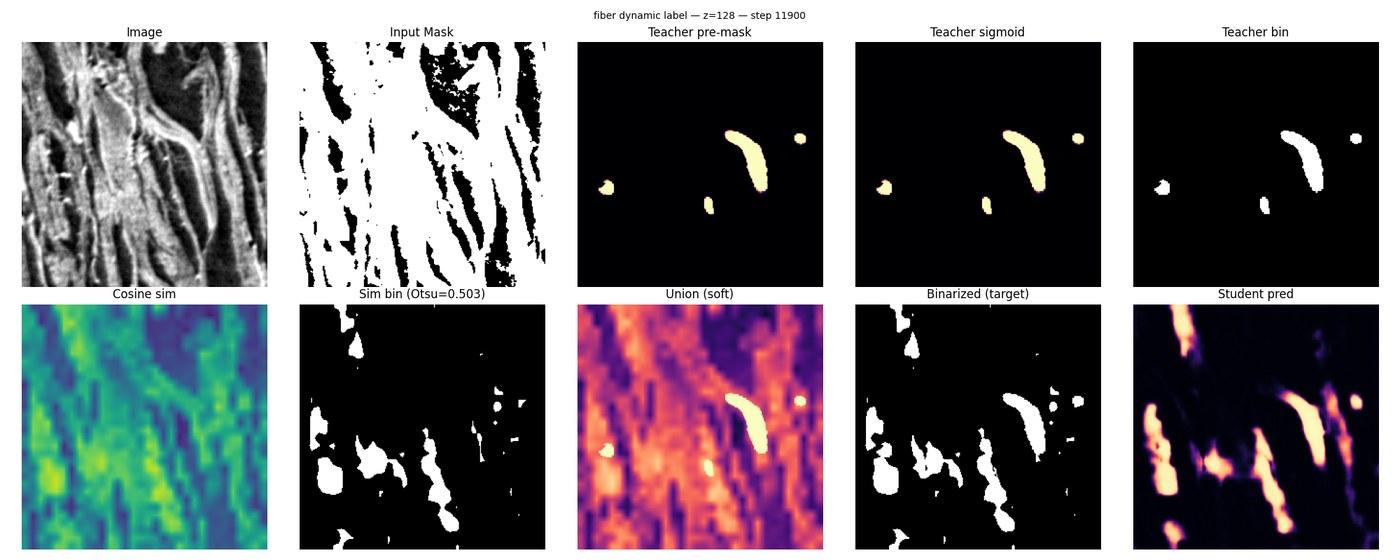
Top row: the raw CT image; the input mask; the teacher's pre-mask; the teacher's sigmoid output; the teacher binarized. Bottom row: the cosine-similarity map; the same map binarized by Otsu's method (labeled "Sim bin (Otsu=0.503)" in the original figure — 0.503 is simply this step's dynamically computed threshold, not a fixed setting); the soft union of the two signals; the binarized training target; and the student's own prediction.
Direct 3D ink segmentation
In recent high-resolution scans of PHerc. Paris 4, ink-bearing deposits become visible enough to support direct volumetric segmentation (see this paper).
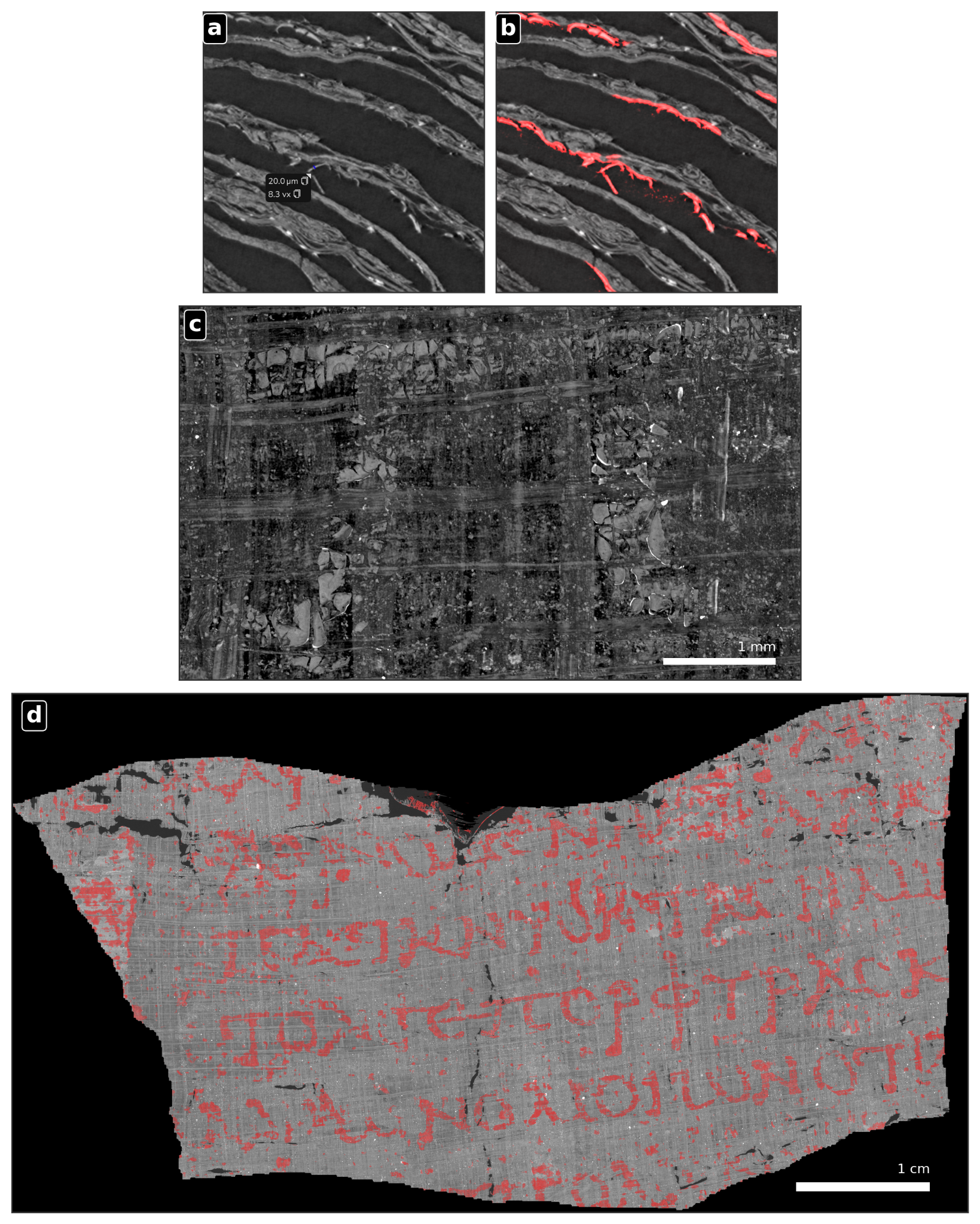
Not every scroll will behave like PHerc. Paris 4 — but direct 3D ink segmentation is possible under favorable scan and preservation conditions, and it gives us a cleaner target for future models.
The checkpoint behind panel (d) in the previous image, ink_3d_dino_guided is trained specifically for PHerc. Paris 4 and is released on Hugging Face.
Careful! The 3D UNet segmentation model for ink segmentation was not only DINO guided, but it also used self-distillation from another 3D ink detection model (not discussed here) to clean up the DINO embedding during UNet training.
If you work in 3D deep learning — segmentation, self-supervised learning, U-Nets — this is a natural fit. When ink is visible or can be localized confidently, as in PHerc. Paris 4 above, the cleanest formulation is voxel-level ink segmentation: it could reduce the ambiguity that 2D-projected labels otherwise introduce, giving the model a direct target instead of an indirect one.
Self-distillation without ground truth
Not every fiber- and ink-modeling effort in this pipeline starts from labels at all. A trainer at scripts/fiber_5class/, specifically its label_generator.py, trains a 3D U-Net for 4-class semantic segmentation — background, vertical fiber, horizontal/angular fiber, and ink — directly on raw CT, with no ground-truth labels of any kind (in PHerc. Paris 4).
Instead, two already-trained teacher networks generate the labels themselves. A teacher, here, is simply an ordinary, already-trained 3D U-Net — one estimating fiber probability, one estimating ink probability — kept completely frozen (its weights are never updated during this training run). Both teachers generate a fresh pseudo-label for every training crop, live, entirely on the GPU, and a student network is trained to reproduce it. Training a network this way — to reproduce another model's output rather than a hand-made label — is called self-distillation.
Each training crop's label is assembled in five steps, confirmed by reading label_generator.py:
- The fiber and ink teachers each produce a voxelwise probability map.
- The fiber probability map is thresholded into a fiber mask and run through a GPU watershed-from-minima — an image-processing technique that floods an image outward from its low points until separately-flooded regions meet, the way water fills separate basins in a landscape. Here, it splits touching or crossing fibers into distinct instances.
- A principal component analysis (PCA) on each instance's own voxel coordinates finds its dominant axis: instances running mostly vertically become class 1 (vertical fiber); everything else becomes class 2 (horizontal/angular fiber).
- The ink teacher's probability map overrides the fiber classes wherever it's confident — ink wins over fiber, becoming class 3.
- Voxels too dark in the raw, pre-augmentation scan are forced back to class 0 (background) regardless of what either teacher said, as a final safety guard.
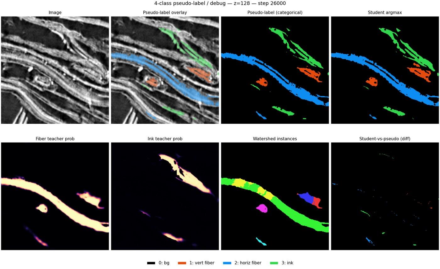
Top row: the raw CT crop, cutting across several parallel fiber bundles; the pseudo-label overlaid on it; the pseudo-label alone; and the student model's own prediction, which closely tracks it. Bottom row: the fiber teacher's probability map, dominated by one long fiber bundle; the ink teacher's probability map, showing two distinct elongated streaks rather than one ambiguous blob; the watershed instances before the vertical/horizontal PCA split — each color is one instance, now legibly separated, including two compact, cleanly isolated cross-sections where a fiber runs roughly vertically through the slice; and the difference between the student's prediction and the pseudo-label it was trained on, mostly black, meaning close agreement. Legend: 0 = background, 1 = vertical fiber, 2 = horizontal fiber, 3 = ink.
The result is released as fiber_ink_4class_selfdistill, alongside the frozen fiber teacher that helped produce it, fiber_selftrain_teacher_epoch30.
Six ways you can help, recapped
Sections 2 and 3 above introduced mesh tracing, approximate labels, fiber connectivity, and 3D ink segmentation — and along the way, six 🙋 callouts pointed out where the community can make the most difference:
- Create datasets with labels better localized on the papyrus’ recto or train ML models that can better preserve the sheets’ topology (See the 🙋 callout in "Surface prediction", Section 2.)
- If you know classical geometry, optimization, or C++: help with building tools that avoid mesh-tracing errors like holes, mergers, and sheet switches without a human checking and fixing every traced piece of surface by hand. (See the 🙋 callout in "Meshes: adding connectivity", Section 2.)
- If you have experience with 3D annotation, active learning, or data-quality work: help improve surface supervision. The labels 3D models learn from are still approximate, and a smaller set of precise labels in the hardest regions may matter more than a larger set of easy ones. (See the 🙋 callout in "Label quality: one of the main unwrapping bottlenecks", Section 2.)
- If you know classical computer vision or fiber/curve-following techniques: help with conservative fiber tracing — following individual papyrus fibers reliably across long distances to give the pipeline connectivity clues it otherwise lacks. (See the 🙋 callout in "Fibers as connectivity clues", Section 2.)
- Devise better evaluation suites and loss functions to improve the global spiral fit, or find efficient and automated ways to introduce exploitable prior information.
- If you work in 3D deep learning (segmentation, self-supervised learning, U-Nets): help with direct 3D ink segmentation, or with self-supervised representation learning that could sharpen nearly every stage of the pipeline at once. (See the 🙋 callout in "Direct 3D ink segmentation", Section 3; self-supervised learning as a cross-cutting direction is discussed further)
5. Bottlenecks
The pipeline works, but not without a person checking its output at almost every stage — and it keeps failing in the same handful of spots.
| Bottleneck | What it means | Current approach | What would help |
|---|---|---|---|
| Compressed or highly curved regions | Some regions lose effective separability between layers. | Better scan regimes, smaller voxel size, shorter propagation distance, phase retrieval. | Scan-quality metrics, and scroll-specific acquisition recipes. |
| No built-in connectivity | CT gives voxels, not sheets or graphs. | Surface prediction plus mesh tracing. | Better geometry priors, fiber tracing, and topology-aware tools. |
| Approximate surface labels | Human-created meshes are useful but not voxel-exact. | Train 3D surface models from approximate annotations. | Label snapping, active learning, self-supervised approaches. |
| Sheet switches | Meshes can jump from one wrap to another. | VC3D inspection and manual correction. | Smarter surface tracing algorithms that avoid introducing sheet switches. |
| Ink depth ambiguity | Fragment photos give 2D labels, not exact 3D ink positions. | Surface-conditioned 3D input with 2D output. | Direct 3D ink segmentation where possible. |
| Cross-scroll generalization | Ink models may work on one scroll but not another. | Fragment training plus scroll-specific pseudo-labeling. | Multi-scroll training, better labels, stronger diagnostics. |
| Data scale | Scroll volumes are too large for ordinary local workflows. | OME-Zarr, chunked processing, cloud storage. | Reproducible streaming pipelines and cheaper compute/storage paths. |
One step forward on cross-scroll generalization came from an unusual source: an autonomous agent swarm, inspired by the open-source karpathy/autoresearch project (released March 2026) and adapted internally for ink-detection model architectures. Running several agents continuously, the system found a configuration that nearly doubled the validation Dice score (computed on pseudo-labels) on PHerc. 1667 while training only on PHerc. 139 data — a genuine cross-scroll generalization improvement.
6. What’s next?
We cant claim final victory. What's changed is that the bottlenecks are now much clearer.
We know that a sealed Herculaneum scroll can be virtually unwrapped and read. We know that high-resolution scanning can make previously elusive ink more visible. We know that direct volumetric ink segmentation is possible in favorable cases. We know that fragment-trained models can generalize far enough to bootstrap scroll-specific reading. We know that semi-automated geometry tools can drastically accelerate tracing, even though human correction remains necessary.
But the next goal is harder to name than any single breakthrough: making all of this reliable, on any scroll, without someone catching every failure.
Can we choose scan parameters that preserve useful signals across scrolls? Can we infer surfaces from voxels without months of correction? Can we reduce the dependence on approximate labels, and reliably tell "no ink" apart from "no ink recovered yet"? And can we make the whole workflow reproducible enough for collection-scale reading?
With the help of the community, we are confident that we can drive these points home. The target of the Vesuvius Challenge for June 2027 is to demonstrate that these questions have a positive answer. And whomever will provide that answer will win prizes, obtain eternal glory and write history with us.
Appendix A: Methods we tried
Not every method in the villa monorepository is production-ready or actively growing. Two neural approaches to tracing were put “on-hold”.
Neural tracer — extrapolation mode. The neural tracing system supports two related displacement-prediction approaches: a "copy" mode (already described above, in Copy Out/In) and an "extrapolation" mode, which instead predicts how the surface displaces as it grows outward beyond its current edge, without reference to a neighboring wrap.
Neural mesh autoregression. Rather than proposing individual candidate points for the classical optimizer, this approach treats a tifxyz surface as a 2D lattice of 3D vertices and predicts an entire continuation of that lattice, one vertex at a time, conditioned on frozen 3D DINO features and a narrow "frontier" band of already-known geometry. Its own documentation calls it "a first MVP,". It is not currently wired into the production GrowPatch tracing loop: it generates mesh patches as a standalone alternative rather than feeding candidates into the classical geometric optimizer. The code lives at neural_tracing/autoreg_mesh.
Slow inference and rollout drift, for both. Two severe limitations apply to both approaches above, independent of the method-specific caveats already noted. Inference is slow at the 2.4 µm resolution the pipeline runs at, for both the neural tracer and the autoregressive mesh model. And running either model over a multi-step rollout — feeding each step's predicted geometry back in as the input to the next step, rather than making one isolated prediction — surfaces a drift problem: small errors compound across steps instead of staying bounded. That matters more than it might sound, because a long, multi-step rollout is the regime real production use needs: tracing a large, continuous span of a scroll, not one isolated local step. Neither problem is solved yet.
Appendix B: Surface morphology and ink signal
An optical profilometer can image a fragment in a way that resembles a photograph, but instead of recording color, each pixel records surface height. The result is a heightmap: a high-resolution map of the fragment’s topography.
Studies on opened Herculaneum fragments show that this surface shape alone carries usable information for telling inked regions from uninked ones. The finding comes from training machine learning models on three-dimensional optical profilometry of mechanically opened fragments (Angelotti, Nicolardi, Henderson & Seales, 2026 — see References), which also measured how detection quality degrades as the lateral resolution of the height-map is coarsened: a direct, empirical link between spatial resolution and how much of the morphological ink signal survives. But ink doesn't always show up as simple raised relief — the signal is more subtle and heterogeneous, and may depend on fine texture, local roughness, cracks, deposits, deformation, or other small-scale surface changes.
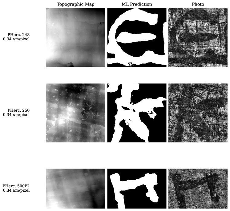
High effective resolution matters here too: some ink information may live at very small spatial scales. That's one more argument for smaller voxel sizes and better phase-retrieval regimes — and a reminder that no single contrast mechanism explains every scroll.
References and implementation links
Publications
- G. Angelotti, S. Parsons, F. Nicolardi, Y. Nader, S. Johnson, D. Josey, P. Henderson, H. Schilling, J. Rudolph, F. McDonald, E. R. Dal Prá, P. Tafforeau, A. Mirone, C. S. Parker, J. P. Posma, B. Kyles, C. Vergara, A. Lavorante, R. Villa, M. C. Robustelli, M. D'Angelo, G. Del Mastro, M. McOsker, K. Fleischer, C. Chapman, N. Friedman, and W. B. Seales, "Complete virtual unwrapping and reading of a rolled Herculaneum papyrus," arXiv:2606.29085, 2026. https://arxiv.org/abs/2606.29085
- G. Angelotti, F. Nicolardi, P. Henderson, and W. B. Seales, "Ink Detection from Surface Topography of the Herculaneum Papyri," Scientific Reports, 2026. https://www.nature.com/articles/s41598-026-58467-1
- S. Parsons, C. S. Parker, C. Chapman, M. Hayashida, and W. B. Seales, "EduceLab-Scrolls: Verifiable Recovery of Text from Herculaneum Papyri using X-ray CT," arXiv:2304.02084, 2023. https://arxiv.org/abs/2304.02084
Methods cited
- nnU-Net — F. Isensee, P. F. Jaeger, S. A. A. Kohl, J. Petersen, and K. H. Maier-Hein, "nnU-Net: a self-configuring method for deep learning-based biomedical image segmentation," Nature Methods 18:203-211, 2021. https://doi.org/10.1038/s41592-020-01008-z (preprint: arXiv:1809.10486)
- U-Net — O. Ronneberger, P. Fischer, and T. Brox, "U-Net: Convolutional Networks for Biomedical Image Segmentation," MICCAI 2015. https://arxiv.org/abs/1505.04597
- 3D U-Net — Ö. Çiçek, A. Abdulkadir, S. S. Lienkamp, T. Brox, and O. Ronneberger, "3D U-Net: Learning Dense Volumetric Segmentation from Sparse Annotation," MICCAI 2016. https://arxiv.org/abs/1606.06650
- ResNet3D pretraining — K. Hara, H. Kataoka, and Y. Satoh, "Can Spatiotemporal 3D CNNs Retrace the History of 2D CNNs and ImageNet?," CVPR 2018. https://arxiv.org/abs/1711.09577
- Kinetics-700 — J. Carreira, E. Noland, C. Hillier, and A. Zisserman, "A Short Note on the Kinetics-700 Human Action Dataset," arXiv:1907.06987, 2019. https://arxiv.org/abs/1907.06987
- DINO — M. Caron, H. Touvron, I. Misra, H. Jégou, J. Mairal, P. Bojanowski, and A. Joulin, "Emerging Properties in Self-Supervised Vision Transformers," ICCV 2021. https://arxiv.org/abs/2104.14294
- Adam optimizer — D. P. Kingma and J. Ba, "Adam: A Method for Stochastic Optimization," ICLR 2015. https://arxiv.org/abs/1412.6980
- Ceres Solver — S. Agarwal, K. Mierle, and the Ceres Solver Team, "Ceres Solver" (software), 2023. http://ceres-solver.org
- SLIM (Scalable Locally Injective Mappings) — M. Rabinovich, R. Poranne, D. Panozzo, and O. Sorkine-Hornung, "Scalable Locally Injective Mappings," ACM Transactions on Graphics 36(2), 2017. https://igl.ethz.ch/projects/slim/
- Phase retrieval (Paganin method) — D. Paganin, S. C. Mayo, T. E. Gureyev, P. R. Miller, and S. W. Wilkins, "Simultaneous phase and amplitude extraction from a single defocused image of a homogeneous object," Journal of Microscopy 206(1):33-40, 2002. https://pubmed.ncbi.nlm.nih.gov/12000561/
- WebKnossos — K. M. Boergens, M. Berning, T. Bocklisch, et al., "webKnossos: efficient online 3D data annotation for connectomics," Nature Methods 14:691-694, 2017. https://doi.org/10.1038/nmeth.4331
- OME-Zarr / OME-NGFF — J. Moore, C. Allan, S. Besson, et al., "OME-NGFF: a next-generation file format for expanding bioimaging data-access strategies," Nature Methods 18:1496-1498, 2021. https://doi.org/10.1038/s41592-021-01326-w (spec: https://ngff.openmicroscopy.org/)
Competition
- Vesuvius Challenge – Surface Detection (Kaggle competition): overview · 1st-place writeup · 5th-place writeup
Code
- villa monorepository (VC3D / Volume Cartographer, lasagna, neural tracing): https://github.com/ScrollPrize/villa
- VC3D / Volume Cartographer app code: https://github.com/ScrollPrize/villa/tree/main/volume-cartographer/apps/src
- lasagna code: https://github.com/ScrollPrize/villa/tree/main/lasagna · lasagna fiber tracer: atlas.py
- Spiral fit code: fit_spiral.py
- Ink detection inference code: ink-detection/optimized_inference
- Neural tracing inference service (heatmap / dense-displacement / copy modes): trace_service.py
- Neural mesh autoregression (MVP): neural_tracing/autoreg_mesh
- 3D DINO implementation: https://github.com/ScrollPrize/villa/tree/main/dinovol
- ScrollFiesta, community automatic mesher: https://github.com/Hob3rMallow/scrollfiesta_public